Feature Stores for Prediction Markets: Fresh Prices, Better Backtests
Feature Stores for Prediction Markets: Fresh Prices, Better Backtests
Feature Stores for Prediction Markets: Fresh Prices, Better Backtests
Build prediction market feature stores with canonical IDs, price freshness budgets, point in time joins, and backfills for reproducible quant research.

Feature Stores for Prediction Markets: Fresh Prices, Better Backtests
Feature store prediction data is the materialized, point-in-time correct feature layer a model consumes for training and inference, defined once in a feature registry so the same logic powers both. The payoff is consistency: no data leakage in training sets, and no training-serving skew in production. Here we cover architecture, temporal joins, freshness, and the operating practices we use at Assymetrix.
TL;DR:
Build training rows with an as of join that selects each feature’s latest value at or before the label timestamp, then test post label changes.
Set a separate freshness limit for each feature by injecting staleness in backtests, then refresh features first when their age degrades model accuracy most.
Use the offline store for backtests and scheduled scoring; live decisions need online reads that return feature age and support explicit fallbacks or abstention.
Across venues, map markets and outcomes to canonical IDs before aggregation, normalize prices and clocks, and keep absent venue values null with an indicator.
Assymetrixdata.assymetrix.comBuild Features From Unified Market DataAssymetrix brings real-time and historical data from Polymarket, Kalshi, and Limitless together through one Data API integration.Explore the Data API
Table of Contents
What is a feature store, and how does it relate to prediction data?
Why do feature stores matter for predictions?
What are the core components of a feature store?
How does point-in-time correctness prevent data leakage?
How do freshness budgets and accuracy-aware scheduling reduce skew?
Should you use batch or online serving for prediction data?
How should you maintain, monitor, and version features?
How do feature-store practices apply to prediction market data?
What security and access controls does market intelligence data need?
How do you combine multiple venues’ data into unified features?
How do you monitor feature data quality for prediction markets?
How do feature stores scale for large prediction market datasets?
How do you handle real-time and historical signals in one feature store?
How we apply feature-store principles at Assymetrix
How to get prediction-market-ready feature data from our Data API
Sources
What is a feature store, and how does it relate to prediction data?
A feature is a transformed datum with predictive power: a rolling 15-minute volume, a spread between two venues, a wallet’s realized hit rate. A feature store is the platform that stores, documents, discovers, and serves those transformed values. Raw data tells you what happened. A feature tells the model what that history means.
The distinction matters for prediction systems because raw sources are poor model inputs. An order book is a stream of mutable states, a trade tape is an append-only log, and a market resolution may arrive well after the activity it labels. None of these is directly consumable. A model wants a row per entity and timestamp, with values computed under rules that never change between experiments. General overviews such as the MLRun feature store documentation describe the same split: a registry for definitions, an offline store for history, an online store for low-latency reads.
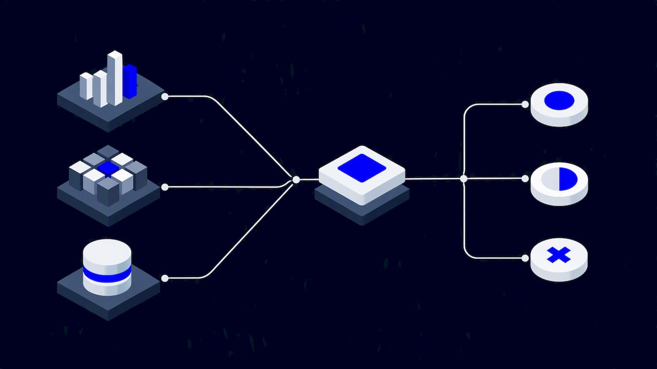
A simple data flow looks like this:
Ingestion: raw trades, quotes, and resolutions land in an append-only event layer with source timestamps preserved.
Transform: feature views compute aggregates, ratios, and lags keyed by a stable entity ID and an event time.
Offline store: the full history of computed feature values is retained for training sets and backtests.
Online store: only the latest value per entity is kept for reads at inference time.
Consumption: training jobs read from the offline store through temporal joins, while live models and agents read from the online store.
The key property is that one transformation definition feeds both stores. When you write the logic twice, once in a notebook for training and once in a service for serving, the two copies drift. That drift is the problem a feature store exists to remove, and the next section explains why it is so expensive.
Why do feature stores matter for predictions?
Prediction quality depends less on model architecture than on whether the model sees at inference the same kind of input it saw in training. Feature stores make that equivalence enforceable rather than aspirational.
Training-serving skew is the gap between how a feature is computed in the training pipeline and how it is computed in production. Typical causes are a rolling window implemented with different boundaries, a null handled as zero in one path and as a missing value in the other, or a unit mismatch between a batch job and a streaming job. Platforms such as the Databricks Feature Store frame this as the primary motivation: define features once in a registry so identical logic materializes into both the offline and online stores.
Beyond skew, three benefits compound over time:
Discovery and reuse: a searchable registry means a quant building a resolution-timing model finds the existing spread and liquidity features instead of rebuilding them with slightly different definitions.
Governance: each feature has an owner, a description, a data source, and a version, so changes are reviewed instead of silently shipped.
Reproducibility: with lineage from raw event to materialized value, you can rerun a past backtest and get the same training rows.
Reuse deserves emphasis. In prediction market work, many models share a common core: implied probability, bid-ask spread, depth near the touch, time to resolution. If each researcher recomputes those with private code, two models that look correlated may simply be disagreeing about how to compute spread. A shared registry turns those disagreements into one reviewed definition.
Reproducibility is the quiet benefit. Research that cannot be rerun cannot be trusted, and a backtest whose features were recomputed ad hoc is closer to an anecdote than to evidence. Our guide to feature engineering for prediction markets lists concrete predictors that benefit from this treatment.
What are the core components of a feature store?
Four components do the structural work: the feature registry, the offline store, the online store, and the feature views or tables that connect them.
Feature registry. The registry holds canonical feature definitions and metadata: name, entity, data type, transformation, owner, freshness expectations, and version. It exposes discovery APIs so people and pipelines can find features by entity or tag. It is also where lineage lives, linking each feature to its upstream sources.
Offline store. This is the historical, materialized record of feature values over time, usually columnar storage on object storage or a warehouse. It serves training sets and backtests. The critical design choice is that it retains every value with its effective timestamp, not just the latest one, because point-in-time joins need the history.
Online store. A low-latency key-value store holding the most recent feature values per entity. Reads here must return with low latency to be usable in live trading logic or an agent loop. If your latency target is tight, the trade-offs in this engineering comparison of vector databases around latency, cost, and atomicity apply to online store selection as well.
Feature views and tables. A feature view is a declarative definition: entity key, event timestamp column, transformation, and the stores to materialize into. Materialization pipelines run the transformation and write results to both stores.
Practical constraints show up quickly:
Key design: the entity key must be stable across sources. For prediction markets that means a canonical market or outcome ID rather than a venue-specific slug.
Time columns: every row needs an event timestamp (when the value was true) and ideally an ingestion timestamp (when you learned it). Without both, you cannot reason about leakage.
Materialization cadence: each view declares how often it refreshes, which feeds directly into freshness budgets covered below.
Idempotent pipelines: reruns of a window must produce identical rows, or backfills corrupt history.
Pro Tip: Store both the event time and the ingestion time on every feature row. Event time lets you join correctly; ingestion time lets you audit what the system actually knew at any moment.
How does point-in-time correctness prevent data leakage?
Point-in-time correctness means that when you build a training row for a label observed at time T, every feature value in that row is the latest value that was available at or before T. Any value computed or updated after T must be excluded. Violating this lets the model peek at the future, producing backtests that look excellent and live results that do not.
The mechanism is a temporal join, also called an AS-OF join. Instead of matching on exact timestamps, which almost never line up, the join finds for each label row the most recent feature row whose timestamp does not exceed the label’s timestamp. The Databricks documentation on point-in-time feature joins describes this: you declare a timestamp key on the feature table, and training set creation uses a timestamp lookup key from your labeled dataframe to perform the match. The same pattern exists outside feature stores; DuckDB’s AS-OF join write-up shows how fuzzy temporal lookups work at query time.
Prediction markets make leakage unusually easy. A market’s final price converges toward 0 or 1 as resolution nears, so any feature that accidentally includes post-event information, a resolved flag, or a late snapshot looks magically predictive. Features computed over a window that extends past the label time are the most common offender.
A practical implementation checklist:
Add a timestamp key to every feature table, representing when the value became true, and a matching lookup timestamp to every label row.
Use the platform’s point-in-time lookup rather than hand-rolled merges. Hand-written joins on a date column silently lose the intraday ordering.
Mind window boundaries: a feature aggregated over a trailing window must close at or before the label time, not at the end of the day.
Test with a controlled example: create a feature that deliberately changes after the label time, build the training set, and assert the later value never appears.
Compare offline to online: replay a handful of historical timestamps through the online path and confirm the values match the offline join.
The controlled leakage test is the one teams skip, and it is the one that catches real bugs. Write it once, run it in continuous integration, and every new feature view inherits the protection.
How do freshness budgets and accuracy-aware scheduling reduce skew?
Staleness is skew in slow motion. If the online store serves a feature that was computed minutes ago while training assumed values current as of the label time, the model sees a different distribution in production than it learned. Common skew sources include:
Stale features: materialization lagging behind the stream, so the online value trails reality.
Delayed labels: resolutions that arrive late, shifting which rows are usable for training.
Precision mismatch: a price rounded to cents in serving but kept at full precision in training.
Null handling differences: missing values imputed one way offline and another way online.
Window misalignment: batch windows aligned to midnight versus streaming windows aligned to the event.
Chasing zero staleness is expensive and usually unnecessary. A more disciplined approach is to quantify how stale each feature can be before it hurts predictions. Recent research on feature freshness budgets for real-time ML inference under stream lag recommends exactly this:
Practitioners should use per-feature freshness budgets, a quantified threshold of how long a feature can be stale before it meaningfully harms prediction accuracy, instead of aiming for perfect real-time consistency. A budget turns “as fresh as possible” into an engineering target you can monitor and spend deliberately.
To set a budget, inject artificial staleness into a feature during backtesting and measure the degradation in your metric. A midpoint price feature for a liquid election market may tolerate a few seconds, while a wallet-level skill score may tolerate hours. The budget is the point where the curve bends.
Once budgets exist, scheduling becomes an optimization problem. Recomputing everything at the tightest cadence wastes compute on features that barely move predictions. The RALF system for accuracy-aware scheduling orchestrates updates using downstream error feedback, prioritizing recomputation where it reduces model error most, which lowers compute cost while maintaining accuracy.
The practical translation:
Assign each feature view a budget and alert when observed age exceeds it.
Rank features by sensitivity: those whose staleness most degrades accuracy refresh first.
Feed model error back into the scheduler so a spike in residuals triggers refreshes for the features most correlated with that error.
Spend slack elsewhere: features with generous budgets run on cheaper, slower schedules.
The result is a system where freshness is a measured resource with a price, not a vague aspiration.
Should you use batch or online serving for prediction data?
The choice follows from the decision you are supporting. Batch scoring suits backtests, nightly portfolio reviews, bulk ranking of markets, and any workload where the answer is consumed minutes or hours later. Online serving is required when a decision depends on the current state: a trading bot reacting to a price move, or an AI agent deciding whether to quote.
The trade-offs are concrete:
Latency versus freshness: online reads return fast but reflect the last materialization, which can trail the live stream by a lag you must measure.
Cost: keeping a low-latency store populated and a streaming pipeline running costs more than a scheduled batch job.
Join complexity: batch scoring over historical data uses the same point-in-time joins as training, so correctness is straightforward. Online serving sidesteps joins by reading the latest value, but then correctness depends on materialization discipline.
Timeliness: batch results are only as current as the last run.
Three design patterns handle the awkward middle:
Cached features: keep recently read values in process memory with a short expiry, cutting read load for hot markets.
Approximate lookups: when exact current values are unavailable, serve the most recent value with its age attached, and let the model or policy decide whether to trust it.
Explicit fallbacks: when a feature is missing or exceeds its freshness budget, fall back to a coarser feature, a default, or a decision to abstain.
The fallback rule matters most. A model that silently consumes a stale value behaves worse than one that knows the value is stale. Return the feature along with its age, and make abstaining a legitimate output.
For live consumers the feed matters as much as the store. Our notes on real-time prediction market data for algorithmic systems cover data delivery, and feeding prediction market data into an AI trading agent covers the consumer side.
How should you maintain, monitor, and version features?
A feature store is infrastructure, and infrastructure decays unless someone watches it. Four disciplines keep prediction features trustworthy.
Distribution monitoring: track each feature’s distribution against a baseline window and alert on shifts in mean, variance, null rate, and quantiles. A sudden jump in null rate usually means an upstream schema change, not a market event.
Lineage: record the path from raw event to materialized value so that when a number of looks wrong you can walk back to the source rows and the transformation version that produced it.
Versioning: treat feature definitions like code. A change to a window length creates a new version, and models pin the version they were trained on.
Controlled backfills: recomputing history is sometimes necessary after a bug fix, but it changes the data under existing experiments. Plan backfills with an explicit window, estimate the compute cost, and write results to a new version rather than overwriting.
Versioning and backfills interact. If you fix a bug in a spread calculation and overwrite history, every earlier experiment becomes irreproducible. If you write a new version, old experiments keep running against the old one and new ones adopt the fix deliberately.
Pro Tip: Pin the feature version in the model’s training metadata. When a result needs to be reproduced or audited, the version string tells you exactly which definitions and which data produced it.
Our walkthrough of three prediction market datasets in one reproducible workflow shows snapshotting and backfill practice end to end.
How do feature-store practices apply to prediction market data?
Prediction markets add specific pressures to general feature-store guidance, and they are the pressures we deal with when aggregating real-time and historical data across Polymarket, Kalshi, and Limitless.
Canonical IDs come first. The same real-world event appears on several venues under different identifiers, titles, and outcome structures. A feature keyed on a venue-specific slug cannot be joined across venues, and a cross-venue spread feature is impossible without a stable mapping. A canonical market and outcome ID is the entity key that makes everything else work.
Timestamps come second. Venues report time differently: block time, matching-engine time, API response time. A feature store only delivers point-in-time correctness if every event carries a consistent timestamp on a common clock, with ingestion time recorded separately.
Freshness budgets should be set per feature class. Price snapshots and order-flow imbalance used in live trading models need tight budgets, while slower features such as trader skill scores and long-window volume aggregates tolerate much more.
For reproducible research, prepare historical snapshots as canonicalized datasets: fixed schema, versioned, with the as-of timestamp preserved. A quant should be able to rerun a backtest against the same snapshot a year later and obtain identical rows. Backfilling the full history under a canonical schema, rather than patching it venue by venue, is what makes that practical.
What security and access controls does market intelligence data need?
Market intelligence data is sensitive even when the underlying prices are public. Derived features such as wallet-level skill scores, Smart Money flags, and proprietary signals carry competitive value, and a feature store concentrates them in one place.
Controls to put in place:
Role-based access at the feature view level: grant read access per view or per tag, so a research group sees what it needs and nothing more.
Separation of definition and consumption rights: analysts can read features, but only owners can change a definition or trigger a backfill.
Credential hygiene for online stores: short-lived, scoped credentials for serving paths, since the online store is reachable from production systems and agents.
Audit logging: record who read, wrote, or redefined which feature and when, using the same lineage metadata the registry already holds.
Environment isolation: keep experimental feature views apart from production ones so a research mistake cannot overwrite served values.
Licensing awareness: commercial and non-commercial uses of a dataset may carry different terms, and the registry is the natural place to record them.
Least privilege is the working rule. Because features compound sensitive inputs into compact signals, a leaked feature table can reveal more than the raw tape it came from.
How do you combine multiple venues’ data into unified features?
Unification is where most cross-venue pipelines break, and the discipline is mostly about normalization before computation.
Resolve entities first: map every venue’s market and outcome to the canonical ID before any aggregation. Join on that ID, never on titles.
Normalize quoting conventions: express every price as an implied probability on the same scale, and handle fee structures and settlement differences explicitly instead of ignoring them.
Align clocks: convert each venue’s timestamps to one reference, keep the original timestamp, and measure per-venue lag so you know how far apart the venues’ views of the same instant are.
Compute per-venue features, then combine: keep venue-level spread, depth, and volume as separate columns, then derive cross-venue features such as divergence from them. This preserves the ability to debug a single venue.
Handle absent venues: a market that exists on two venues but not a third should yield a null for the third, with an explicit indicator rather than a silently imputed value.
Divergence and arbitrage signals depend on getting these steps right. Our guide to cross-venue prediction market data and canonical IDs walks through the mapping, and the signal generation guide shows how unified features feed downstream signals.
How do you monitor feature data quality for prediction markets?
Generic drift monitoring catches only part of the failure modes. Prediction market feeds fail in characteristic ways, and the alerts should target them.
Staleness against budget: alert when a view’s age exceeds its freshness budget, with severity tied to how sensitive the consuming models are.
Venue silence: alert when a venue’s event rate drops to zero during hours it is normally active, which usually signals a connector fault rather than a quiet market.
Cross-venue sanity checks: implied probabilities for the same canonical outcome should stay within plausible distance of each other, and a sudden persistent gap may be a mapping error rather than an opportunity.
Bounds and invariants: probabilities must lie between 0 and 1, outcome probabilities within a market should sum near 1, and volumes should not be negative.
Resolution handling: watch for features still updating on resolved markets, and for labels arriving outside expected windows.
Offline-online parity: periodically recompute a sample of served values from the offline store and alert on mismatch, which is the direct detector of training-serving skew.
Route alerts by consequence. A freshness breach on a live trading feature should page someone, while a drift warning on a slow research feature can wait for review.
How do feature stores scale for large prediction market datasets?
Prediction market history is large and append-heavy, with trade-level data accumulating into billions of rows. Scale pressures show up in three places.
Partitioning: partition offline tables by event date and canonical market so temporal joins and backfills scan only the relevant slices rather than the whole history.
Columnar, compressed storage: analytical reads touch a few columns across many rows, which columnar formats handle efficiently.
Incremental materialization: compute only new windows rather than recomputing history, reserving full backfills for deliberate, versioned events.
Online store sizing: the online store holds one latest value per entity, so size it by the count of active canonical entities, not by history, and expire resolved markets.
Hot and cold separation: active markets drive most reads, so keep them in fast storage and let resolved markets age into the offline store only.
Join cost: AS-OF joins over very large label sets are the expensive step, so sort by key and time, pre-filter to the label window, and avoid joining unneeded features.
The scale of the historical record is what makes disciplined partitioning non-negotiable. For teams that need deep history, our overview of bulk historical access for reproducible backtests describes what a full backfill involves.
How do you handle real-time and historical signals in one feature store?
The goal is a single definition that serves both a stream and an archive, so a live model and a backtest use identical logic.
One transformation, two executions: express each feature once and run it over the stream for the online store and over archived events for the offline store, validating that both produce matching values on shared windows.
Replay as the bridge: feed historical events through the same code path as the live stream, preserving original event timestamps, so a backtest is a replay rather than a separate implementation.
Late and out-of-order events: decide a watermark policy, accept corrections within it, and record which version of a value the model actually saw.
Backfill without disturbing live reads: write historical recomputations to a separate version, then promote it deliberately.
Different signal types, different handling: order-book snapshots are state, trades are events, and resolutions are labels. Each needs its own time semantics in the view definition, especially labels, which must never leak into feature windows.
Expose the same schema: whether a consumer calls a REST endpoint for the latest value or a bulk export for history, the field names and units should be identical.
That last point is why we publish access paths under one schema. The developer guide covers the API, and the AI agent pipeline notes cover consumption by agents.
How we apply feature-store principles at Assymetrix
We aggregate real-time and historical data across Polymarket, Kalshi, and Limitless into one intelligence layer, and the work that matters most is the least glamorous: canonical IDs and consistent timestamps. Everything in this article depends on them. A temporal join is only as correct as the clocks beneath it, and a cross-venue feature is only as meaningful as the entity mapping behind it.
Our opinion is that most teams underinvest in the plumbing and overinvest in model choice. A modest model on point-in-time correct, canonicalized features will usually beat a sophisticated model trained on leaky, venue-fragmented data, and the leaky version often looks better until it trades live. Doing the normalization and backfill once, centrally, is what lets quants and algorithmic agents spend their time on signals instead of reconciling identifiers.
That is the engineering lift we aim to remove. If you are onboarding as a developer, the Data API documentation is the place to start.
— Dean
How to get prediction-market-ready feature data from our Data API
Our Data API delivers real-time and historical cross-venue prediction market data. Current price details are available on our website.

Ways to get started:
Read the data feed guide for real-time and historical endpoints.
Follow the Python developer guide to load features into your models.
Contact our team through Data.
For quant workflows, the value is reproducibility and speed: historical data for backtests and real-time data for live feature serving, both under one schema. Start with a small canonical subset, validate your point-in-time joins, then widen coverage.
FAQ
What is feature store prediction data?
It is the set of precomputed, versioned feature values a model reads for training and inference, defined once in a registry. Because the same logic fills the offline and online stores, training sets and live predictions see consistent inputs.
How does a feature store prevent data leakage?
It uses point-in-time joins that retrieve the latest feature value at or before each label’s timestamp, as described in the Databricks time-series feature documentation. Values updated after the label time are excluded from the training row.
What is a feature freshness budget?
A freshness budget is a quantified limit on how stale a feature may become before it meaningfully hurts prediction accuracy. Research on freshness budgets recommends setting one per feature instead of chasing perfect real-time freshness.
Do I need an online store for every prediction workload?
No. Batch scoring for backtests and periodic ranking works from the offline store alone. You need an online store when a decision depends on current values, as with live trading bots and agents.
How does accuracy-aware scheduling save compute?
It refreshes features in order of their effect on downstream error rather than on a fixed timer. The RALF scheduler uses model error feedback to prioritize recomputation, lowering cost while maintaining accuracy.
Sources
Feature Stores for Prediction Markets: Fresh Prices, Better Backtests
Feature store prediction data is the materialized, point-in-time correct feature layer a model consumes for training and inference, defined once in a feature registry so the same logic powers both. The payoff is consistency: no data leakage in training sets, and no training-serving skew in production. Here we cover architecture, temporal joins, freshness, and the operating practices we use at Assymetrix.
TL;DR:
Build training rows with an as of join that selects each feature’s latest value at or before the label timestamp, then test post label changes.
Set a separate freshness limit for each feature by injecting staleness in backtests, then refresh features first when their age degrades model accuracy most.
Use the offline store for backtests and scheduled scoring; live decisions need online reads that return feature age and support explicit fallbacks or abstention.
Across venues, map markets and outcomes to canonical IDs before aggregation, normalize prices and clocks, and keep absent venue values null with an indicator.
Assymetrixdata.assymetrix.comBuild Features From Unified Market DataAssymetrix brings real-time and historical data from Polymarket, Kalshi, and Limitless together through one Data API integration.Explore the Data API
Table of Contents
What is a feature store, and how does it relate to prediction data?
Why do feature stores matter for predictions?
What are the core components of a feature store?
How does point-in-time correctness prevent data leakage?
How do freshness budgets and accuracy-aware scheduling reduce skew?
Should you use batch or online serving for prediction data?
How should you maintain, monitor, and version features?
How do feature-store practices apply to prediction market data?
What security and access controls does market intelligence data need?
How do you combine multiple venues’ data into unified features?
How do you monitor feature data quality for prediction markets?
How do feature stores scale for large prediction market datasets?
How do you handle real-time and historical signals in one feature store?
How we apply feature-store principles at Assymetrix
How to get prediction-market-ready feature data from our Data API
Sources
What is a feature store, and how does it relate to prediction data?
A feature is a transformed datum with predictive power: a rolling 15-minute volume, a spread between two venues, a wallet’s realized hit rate. A feature store is the platform that stores, documents, discovers, and serves those transformed values. Raw data tells you what happened. A feature tells the model what that history means.
The distinction matters for prediction systems because raw sources are poor model inputs. An order book is a stream of mutable states, a trade tape is an append-only log, and a market resolution may arrive well after the activity it labels. None of these is directly consumable. A model wants a row per entity and timestamp, with values computed under rules that never change between experiments. General overviews such as the MLRun feature store documentation describe the same split: a registry for definitions, an offline store for history, an online store for low-latency reads.
A simple data flow looks like this:
Ingestion: raw trades, quotes, and resolutions land in an append-only event layer with source timestamps preserved.
Transform: feature views compute aggregates, ratios, and lags keyed by a stable entity ID and an event time.
Offline store: the full history of computed feature values is retained for training sets and backtests.
Online store: only the latest value per entity is kept for reads at inference time.
Consumption: training jobs read from the offline store through temporal joins, while live models and agents read from the online store.
The key property is that one transformation definition feeds both stores. When you write the logic twice, once in a notebook for training and once in a service for serving, the two copies drift. That drift is the problem a feature store exists to remove, and the next section explains why it is so expensive.
Why do feature stores matter for predictions?
Prediction quality depends less on model architecture than on whether the model sees at inference the same kind of input it saw in training. Feature stores make that equivalence enforceable rather than aspirational.
Training-serving skew is the gap between how a feature is computed in the training pipeline and how it is computed in production. Typical causes are a rolling window implemented with different boundaries, a null handled as zero in one path and as a missing value in the other, or a unit mismatch between a batch job and a streaming job. Platforms such as the Databricks Feature Store frame this as the primary motivation: define features once in a registry so identical logic materializes into both the offline and online stores.
Beyond skew, three benefits compound over time:
Discovery and reuse: a searchable registry means a quant building a resolution-timing model finds the existing spread and liquidity features instead of rebuilding them with slightly different definitions.
Governance: each feature has an owner, a description, a data source, and a version, so changes are reviewed instead of silently shipped.
Reproducibility: with lineage from raw event to materialized value, you can rerun a past backtest and get the same training rows.
Reuse deserves emphasis. In prediction market work, many models share a common core: implied probability, bid-ask spread, depth near the touch, time to resolution. If each researcher recomputes those with private code, two models that look correlated may simply be disagreeing about how to compute spread. A shared registry turns those disagreements into one reviewed definition.
Reproducibility is the quiet benefit. Research that cannot be rerun cannot be trusted, and a backtest whose features were recomputed ad hoc is closer to an anecdote than to evidence. Our guide to feature engineering for prediction markets lists concrete predictors that benefit from this treatment.
What are the core components of a feature store?
Four components do the structural work: the feature registry, the offline store, the online store, and the feature views or tables that connect them.
Feature registry. The registry holds canonical feature definitions and metadata: name, entity, data type, transformation, owner, freshness expectations, and version. It exposes discovery APIs so people and pipelines can find features by entity or tag. It is also where lineage lives, linking each feature to its upstream sources.
Offline store. This is the historical, materialized record of feature values over time, usually columnar storage on object storage or a warehouse. It serves training sets and backtests. The critical design choice is that it retains every value with its effective timestamp, not just the latest one, because point-in-time joins need the history.
Online store. A low-latency key-value store holding the most recent feature values per entity. Reads here must return with low latency to be usable in live trading logic or an agent loop. If your latency target is tight, the trade-offs in this engineering comparison of vector databases around latency, cost, and atomicity apply to online store selection as well.
Feature views and tables. A feature view is a declarative definition: entity key, event timestamp column, transformation, and the stores to materialize into. Materialization pipelines run the transformation and write results to both stores.
Practical constraints show up quickly:
Key design: the entity key must be stable across sources. For prediction markets that means a canonical market or outcome ID rather than a venue-specific slug.
Time columns: every row needs an event timestamp (when the value was true) and ideally an ingestion timestamp (when you learned it). Without both, you cannot reason about leakage.
Materialization cadence: each view declares how often it refreshes, which feeds directly into freshness budgets covered below.
Idempotent pipelines: reruns of a window must produce identical rows, or backfills corrupt history.
Pro Tip: Store both the event time and the ingestion time on every feature row. Event time lets you join correctly; ingestion time lets you audit what the system actually knew at any moment.
How does point-in-time correctness prevent data leakage?
Point-in-time correctness means that when you build a training row for a label observed at time T, every feature value in that row is the latest value that was available at or before T. Any value computed or updated after T must be excluded. Violating this lets the model peek at the future, producing backtests that look excellent and live results that do not.
The mechanism is a temporal join, also called an AS-OF join. Instead of matching on exact timestamps, which almost never line up, the join finds for each label row the most recent feature row whose timestamp does not exceed the label’s timestamp. The Databricks documentation on point-in-time feature joins describes this: you declare a timestamp key on the feature table, and training set creation uses a timestamp lookup key from your labeled dataframe to perform the match. The same pattern exists outside feature stores; DuckDB’s AS-OF join write-up shows how fuzzy temporal lookups work at query time.
Prediction markets make leakage unusually easy. A market’s final price converges toward 0 or 1 as resolution nears, so any feature that accidentally includes post-event information, a resolved flag, or a late snapshot looks magically predictive. Features computed over a window that extends past the label time are the most common offender.
A practical implementation checklist:
Add a timestamp key to every feature table, representing when the value became true, and a matching lookup timestamp to every label row.
Use the platform’s point-in-time lookup rather than hand-rolled merges. Hand-written joins on a date column silently lose the intraday ordering.
Mind window boundaries: a feature aggregated over a trailing window must close at or before the label time, not at the end of the day.
Test with a controlled example: create a feature that deliberately changes after the label time, build the training set, and assert the later value never appears.
Compare offline to online: replay a handful of historical timestamps through the online path and confirm the values match the offline join.
The controlled leakage test is the one teams skip, and it is the one that catches real bugs. Write it once, run it in continuous integration, and every new feature view inherits the protection.
How do freshness budgets and accuracy-aware scheduling reduce skew?
Staleness is skew in slow motion. If the online store serves a feature that was computed minutes ago while training assumed values current as of the label time, the model sees a different distribution in production than it learned. Common skew sources include:
Stale features: materialization lagging behind the stream, so the online value trails reality.
Delayed labels: resolutions that arrive late, shifting which rows are usable for training.
Precision mismatch: a price rounded to cents in serving but kept at full precision in training.
Null handling differences: missing values imputed one way offline and another way online.
Window misalignment: batch windows aligned to midnight versus streaming windows aligned to the event.
Chasing zero staleness is expensive and usually unnecessary. A more disciplined approach is to quantify how stale each feature can be before it hurts predictions. Recent research on feature freshness budgets for real-time ML inference under stream lag recommends exactly this:
Practitioners should use per-feature freshness budgets, a quantified threshold of how long a feature can be stale before it meaningfully harms prediction accuracy, instead of aiming for perfect real-time consistency. A budget turns “as fresh as possible” into an engineering target you can monitor and spend deliberately.
To set a budget, inject artificial staleness into a feature during backtesting and measure the degradation in your metric. A midpoint price feature for a liquid election market may tolerate a few seconds, while a wallet-level skill score may tolerate hours. The budget is the point where the curve bends.
Once budgets exist, scheduling becomes an optimization problem. Recomputing everything at the tightest cadence wastes compute on features that barely move predictions. The RALF system for accuracy-aware scheduling orchestrates updates using downstream error feedback, prioritizing recomputation where it reduces model error most, which lowers compute cost while maintaining accuracy.
The practical translation:
Assign each feature view a budget and alert when observed age exceeds it.
Rank features by sensitivity: those whose staleness most degrades accuracy refresh first.
Feed model error back into the scheduler so a spike in residuals triggers refreshes for the features most correlated with that error.
Spend slack elsewhere: features with generous budgets run on cheaper, slower schedules.
The result is a system where freshness is a measured resource with a price, not a vague aspiration.
Should you use batch or online serving for prediction data?
The choice follows from the decision you are supporting. Batch scoring suits backtests, nightly portfolio reviews, bulk ranking of markets, and any workload where the answer is consumed minutes or hours later. Online serving is required when a decision depends on the current state: a trading bot reacting to a price move, or an AI agent deciding whether to quote.
The trade-offs are concrete:
Latency versus freshness: online reads return fast but reflect the last materialization, which can trail the live stream by a lag you must measure.
Cost: keeping a low-latency store populated and a streaming pipeline running costs more than a scheduled batch job.
Join complexity: batch scoring over historical data uses the same point-in-time joins as training, so correctness is straightforward. Online serving sidesteps joins by reading the latest value, but then correctness depends on materialization discipline.
Timeliness: batch results are only as current as the last run.
Three design patterns handle the awkward middle:
Cached features: keep recently read values in process memory with a short expiry, cutting read load for hot markets.
Approximate lookups: when exact current values are unavailable, serve the most recent value with its age attached, and let the model or policy decide whether to trust it.
Explicit fallbacks: when a feature is missing or exceeds its freshness budget, fall back to a coarser feature, a default, or a decision to abstain.
The fallback rule matters most. A model that silently consumes a stale value behaves worse than one that knows the value is stale. Return the feature along with its age, and make abstaining a legitimate output.
For live consumers the feed matters as much as the store. Our notes on real-time prediction market data for algorithmic systems cover data delivery, and feeding prediction market data into an AI trading agent covers the consumer side.
How should you maintain, monitor, and version features?
A feature store is infrastructure, and infrastructure decays unless someone watches it. Four disciplines keep prediction features trustworthy.
Distribution monitoring: track each feature’s distribution against a baseline window and alert on shifts in mean, variance, null rate, and quantiles. A sudden jump in null rate usually means an upstream schema change, not a market event.
Lineage: record the path from raw event to materialized value so that when a number of looks wrong you can walk back to the source rows and the transformation version that produced it.
Versioning: treat feature definitions like code. A change to a window length creates a new version, and models pin the version they were trained on.
Controlled backfills: recomputing history is sometimes necessary after a bug fix, but it changes the data under existing experiments. Plan backfills with an explicit window, estimate the compute cost, and write results to a new version rather than overwriting.
Versioning and backfills interact. If you fix a bug in a spread calculation and overwrite history, every earlier experiment becomes irreproducible. If you write a new version, old experiments keep running against the old one and new ones adopt the fix deliberately.
Pro Tip: Pin the feature version in the model’s training metadata. When a result needs to be reproduced or audited, the version string tells you exactly which definitions and which data produced it.
Our walkthrough of three prediction market datasets in one reproducible workflow shows snapshotting and backfill practice end to end.
How do feature-store practices apply to prediction market data?
Prediction markets add specific pressures to general feature-store guidance, and they are the pressures we deal with when aggregating real-time and historical data across Polymarket, Kalshi, and Limitless.
Canonical IDs come first. The same real-world event appears on several venues under different identifiers, titles, and outcome structures. A feature keyed on a venue-specific slug cannot be joined across venues, and a cross-venue spread feature is impossible without a stable mapping. A canonical market and outcome ID is the entity key that makes everything else work.
Timestamps come second. Venues report time differently: block time, matching-engine time, API response time. A feature store only delivers point-in-time correctness if every event carries a consistent timestamp on a common clock, with ingestion time recorded separately.
Freshness budgets should be set per feature class. Price snapshots and order-flow imbalance used in live trading models need tight budgets, while slower features such as trader skill scores and long-window volume aggregates tolerate much more.
For reproducible research, prepare historical snapshots as canonicalized datasets: fixed schema, versioned, with the as-of timestamp preserved. A quant should be able to rerun a backtest against the same snapshot a year later and obtain identical rows. Backfilling the full history under a canonical schema, rather than patching it venue by venue, is what makes that practical.
What security and access controls does market intelligence data need?
Market intelligence data is sensitive even when the underlying prices are public. Derived features such as wallet-level skill scores, Smart Money flags, and proprietary signals carry competitive value, and a feature store concentrates them in one place.
Controls to put in place:
Role-based access at the feature view level: grant read access per view or per tag, so a research group sees what it needs and nothing more.
Separation of definition and consumption rights: analysts can read features, but only owners can change a definition or trigger a backfill.
Credential hygiene for online stores: short-lived, scoped credentials for serving paths, since the online store is reachable from production systems and agents.
Audit logging: record who read, wrote, or redefined which feature and when, using the same lineage metadata the registry already holds.
Environment isolation: keep experimental feature views apart from production ones so a research mistake cannot overwrite served values.
Licensing awareness: commercial and non-commercial uses of a dataset may carry different terms, and the registry is the natural place to record them.
Least privilege is the working rule. Because features compound sensitive inputs into compact signals, a leaked feature table can reveal more than the raw tape it came from.
How do you combine multiple venues’ data into unified features?
Unification is where most cross-venue pipelines break, and the discipline is mostly about normalization before computation.
Resolve entities first: map every venue’s market and outcome to the canonical ID before any aggregation. Join on that ID, never on titles.
Normalize quoting conventions: express every price as an implied probability on the same scale, and handle fee structures and settlement differences explicitly instead of ignoring them.
Align clocks: convert each venue’s timestamps to one reference, keep the original timestamp, and measure per-venue lag so you know how far apart the venues’ views of the same instant are.
Compute per-venue features, then combine: keep venue-level spread, depth, and volume as separate columns, then derive cross-venue features such as divergence from them. This preserves the ability to debug a single venue.
Handle absent venues: a market that exists on two venues but not a third should yield a null for the third, with an explicit indicator rather than a silently imputed value.
Divergence and arbitrage signals depend on getting these steps right. Our guide to cross-venue prediction market data and canonical IDs walks through the mapping, and the signal generation guide shows how unified features feed downstream signals.
How do you monitor feature data quality for prediction markets?
Generic drift monitoring catches only part of the failure modes. Prediction market feeds fail in characteristic ways, and the alerts should target them.
Staleness against budget: alert when a view’s age exceeds its freshness budget, with severity tied to how sensitive the consuming models are.
Venue silence: alert when a venue’s event rate drops to zero during hours it is normally active, which usually signals a connector fault rather than a quiet market.
Cross-venue sanity checks: implied probabilities for the same canonical outcome should stay within plausible distance of each other, and a sudden persistent gap may be a mapping error rather than an opportunity.
Bounds and invariants: probabilities must lie between 0 and 1, outcome probabilities within a market should sum near 1, and volumes should not be negative.
Resolution handling: watch for features still updating on resolved markets, and for labels arriving outside expected windows.
Offline-online parity: periodically recompute a sample of served values from the offline store and alert on mismatch, which is the direct detector of training-serving skew.
Route alerts by consequence. A freshness breach on a live trading feature should page someone, while a drift warning on a slow research feature can wait for review.
How do feature stores scale for large prediction market datasets?
Prediction market history is large and append-heavy, with trade-level data accumulating into billions of rows. Scale pressures show up in three places.
Partitioning: partition offline tables by event date and canonical market so temporal joins and backfills scan only the relevant slices rather than the whole history.
Columnar, compressed storage: analytical reads touch a few columns across many rows, which columnar formats handle efficiently.
Incremental materialization: compute only new windows rather than recomputing history, reserving full backfills for deliberate, versioned events.
Online store sizing: the online store holds one latest value per entity, so size it by the count of active canonical entities, not by history, and expire resolved markets.
Hot and cold separation: active markets drive most reads, so keep them in fast storage and let resolved markets age into the offline store only.
Join cost: AS-OF joins over very large label sets are the expensive step, so sort by key and time, pre-filter to the label window, and avoid joining unneeded features.
The scale of the historical record is what makes disciplined partitioning non-negotiable. For teams that need deep history, our overview of bulk historical access for reproducible backtests describes what a full backfill involves.
How do you handle real-time and historical signals in one feature store?
The goal is a single definition that serves both a stream and an archive, so a live model and a backtest use identical logic.
One transformation, two executions: express each feature once and run it over the stream for the online store and over archived events for the offline store, validating that both produce matching values on shared windows.
Replay as the bridge: feed historical events through the same code path as the live stream, preserving original event timestamps, so a backtest is a replay rather than a separate implementation.
Late and out-of-order events: decide a watermark policy, accept corrections within it, and record which version of a value the model actually saw.
Backfill without disturbing live reads: write historical recomputations to a separate version, then promote it deliberately.
Different signal types, different handling: order-book snapshots are state, trades are events, and resolutions are labels. Each needs its own time semantics in the view definition, especially labels, which must never leak into feature windows.
Expose the same schema: whether a consumer calls a REST endpoint for the latest value or a bulk export for history, the field names and units should be identical.
That last point is why we publish access paths under one schema. The developer guide covers the API, and the AI agent pipeline notes cover consumption by agents.
How we apply feature-store principles at Assymetrix
We aggregate real-time and historical data across Polymarket, Kalshi, and Limitless into one intelligence layer, and the work that matters most is the least glamorous: canonical IDs and consistent timestamps. Everything in this article depends on them. A temporal join is only as correct as the clocks beneath it, and a cross-venue feature is only as meaningful as the entity mapping behind it.
Our opinion is that most teams underinvest in the plumbing and overinvest in model choice. A modest model on point-in-time correct, canonicalized features will usually beat a sophisticated model trained on leaky, venue-fragmented data, and the leaky version often looks better until it trades live. Doing the normalization and backfill once, centrally, is what lets quants and algorithmic agents spend their time on signals instead of reconciling identifiers.
That is the engineering lift we aim to remove. If you are onboarding as a developer, the Data API documentation is the place to start.
— Dean
How to get prediction-market-ready feature data from our Data API
Our Data API delivers real-time and historical cross-venue prediction market data. Current price details are available on our website.
Ways to get started:
Read the data feed guide for real-time and historical endpoints.
Follow the Python developer guide to load features into your models.
Contact our team through Data.
For quant workflows, the value is reproducibility and speed: historical data for backtests and real-time data for live feature serving, both under one schema. Start with a small canonical subset, validate your point-in-time joins, then widen coverage.
FAQ
What is feature store prediction data?
It is the set of precomputed, versioned feature values a model reads for training and inference, defined once in a registry. Because the same logic fills the offline and online stores, training sets and live predictions see consistent inputs.
How does a feature store prevent data leakage?
It uses point-in-time joins that retrieve the latest feature value at or before each label’s timestamp, as described in the Databricks time-series feature documentation. Values updated after the label time are excluded from the training row.
What is a feature freshness budget?
A freshness budget is a quantified limit on how stale a feature may become before it meaningfully hurts prediction accuracy. Research on freshness budgets recommends setting one per feature instead of chasing perfect real-time freshness.
Do I need an online store for every prediction workload?
No. Batch scoring for backtests and periodic ranking works from the offline store alone. You need an online store when a decision depends on current values, as with live trading bots and agents.
How does accuracy-aware scheduling save compute?
It refreshes features in order of their effect on downstream error rather than on a fixed timer. The RALF scheduler uses model error feedback to prioritize recomputation, lowering cost while maintaining accuracy.
Sources
Other Blog


