Feature Engineering for Devs: 9 Predictors for Prediction Markets
Feature Engineering for Devs: 9 Predictors for Prediction Markets
Feature Engineering for Devs: 9 Predictors for Prediction Markets
Nine starter predictors and timestamped signal patterns for developers and quants building cross venue prediction market models, plus cross‑venue recipes...
Feature Engineering for Devs: 9 Predictors for Prediction Markets
Six feature families consistently separate profitable prediction-market models from noise: price lag and momentum, orderbook microstructure, volume anomalies, time-to-expiry decay, Smart Money wallet entries, and cross-venue spreads. None of them work in isolation, and none of them work well on single-venue data. Cross-venue, timestamped, normalized data is what turns these signals into a tradable edge rather than a backtest artifact, and that is the piece most home-grown pipelines get wrong. A Data API exists that provides developers with a unified feed of trades, orderbook snapshots, OHLCV, and wallet activity across Polymarket, Kalshi, and Limitless without requiring three separate integrations.
TL;DR:
The most predictive features include seven-day price lag and cross-venue spreads, which outperform single-venue signals by exposing market fragmentation.
Cross-venue, timestamped, normalized data significantly enhances model accuracy, and a unified API simplifies data collection from Polymarket, Kalshi, and Limitless.
Preventing feature leakage requires strict timestamp discipline and walk-forward validation, as using pre-resolution data can create misleading backtest results.
A small, well-chosen feature set—such as lagged prices, bid-ask imbalance, and wallet activity—combined with multiple temporal cadences yields reliable initial models.
Proper feature engineering emphasizes reproducibility, interpretability, and realistic validation, with the Brier score commonly used to measure calibration and forecasting accuracy.
AssymetrixBuild With Unified Market DataAssymetrix gives developers and AI agents unified prediction market data across Polymarket, Kalshi, and Limitless through one integration.Explore Assymetrix
Table of Contents
What Feature Categories Actually Predict Resolution Outcomes?
How Do You Engineer Features From Raw Trade and Orderbook Data?
Why Separate the Feature Engine From the Signal Engine?
How Should You Validate Prediction-Market Signals?
How Does a Unified Data API Speed Up Feature Engineering?
What’s a Good Starter Feature Set for a First Model?
Feature Selection and Dimensionality Reduction for Prediction-Market Models
How Do You Interpret Feature Importance in These Models?
What Are the Most Common Feature Engineering Mistakes?
What Does Successful Feature Engineering Look Like in Practice?
Priorities and Pitfalls Worth Repeating
Get Unified Cross-Venue Data Without Building Three Integrations
Sources
What Feature Categories Actually Predict Resolution Outcomes?
Most prediction-market models fail not because of weak algorithms but because of shallow feature sets pulled from a single venue’s price history. The categories below carry the actual signal.
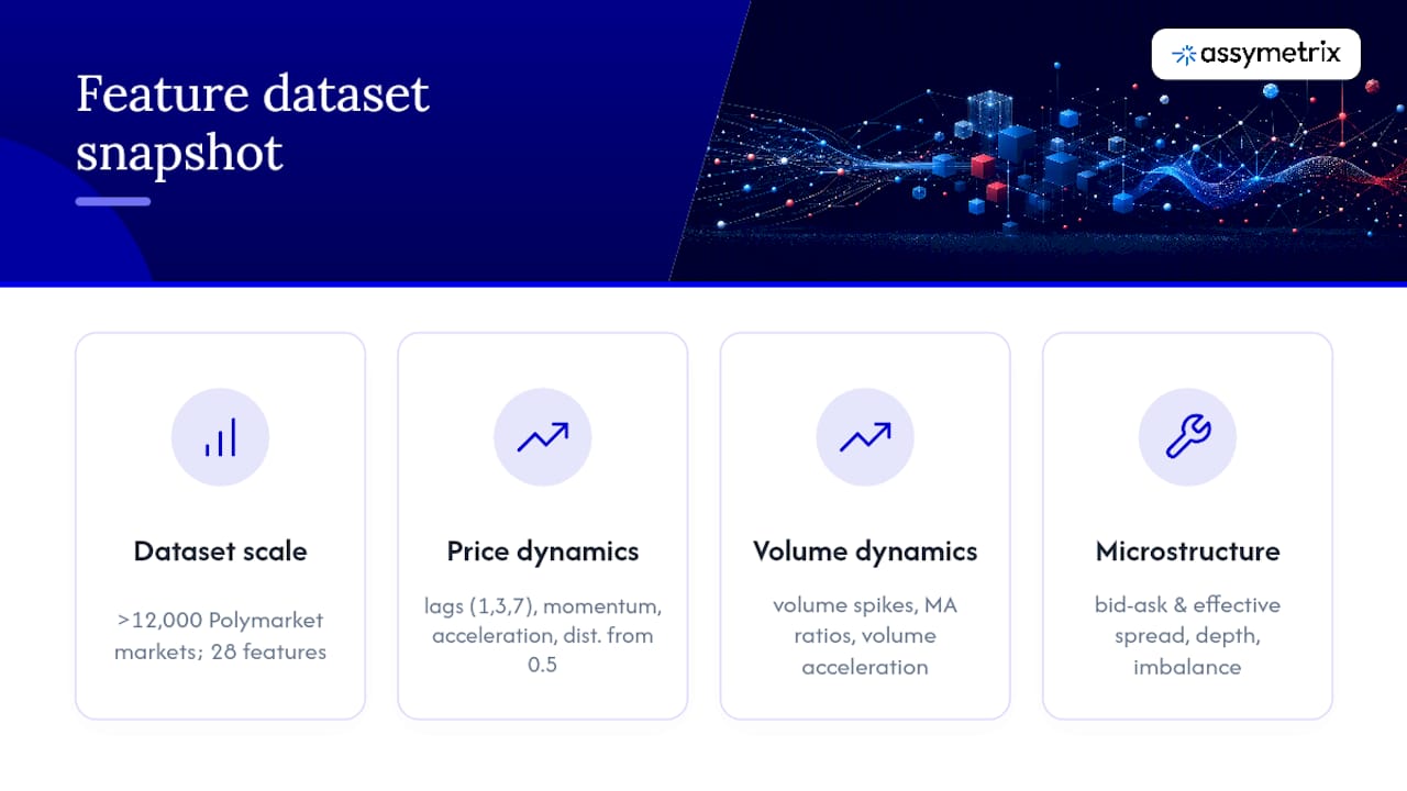
Price dynamics. Lagged prices at 1, 3, and 7 periods, momentum (rate of change), acceleration (second derivative of momentum), and distance from 0.5 all matter, but not equally. A reproduced feature-importance study on a production Polymarket pipeline found that price_lag7 ranked as the single most important predictor for identifying mispriced contracts, ahead of shorter lags and most microstructure inputs.
Microstructure and liquidity. Bid-ask spread, effective spread, order-book depth, and bid-ask imbalance function as proxies for informed trading and execution risk. A wide spread on a thinly traded contract tells you the last print is unreliable; a persistent one-sided imbalance often precedes a directional move before the mid-price adjusts.
Volume dynamics. Volume spikes, volume moving-average ratios, and volume acceleration flag new information hitting the market, often before price fully reflects it.
Temporal features. Hours-to-expiry, time-decay curves, and calendar effects around scheduled resolution events (elections, earnings, Fed meetings) shape how variance behaves as a market approaches settlement. Deadline-resolution structure changes the statistics of the underlying process itself, which is why structural volatility models built around deadline dynamics tend to outperform standard GARCH approaches on these instruments.
Smart Money and trader features. Wallet-entry flags, concentration of top-decile wallets in a market, and trader-skill scores built from historical resolution accuracy.
Cross-venue features. Matched-event price spreads and synthetic Dutch-book cost, which expose fragmentation between venues pricing the same real-world event differently.
A public dataset covering more than 12,000 Polymarket markets and 28 pre-computed features spanning price, volume, and microstructure categories is a useful reference point for what a mature feature table looks like in practice.
How Do You Engineer Features From Raw Trade and Orderbook Data?
Turning raw trades, orderbook snapshots, OHLCV bars, and wallet events into model-ready features follows a repeatable sequence.
Canonicalize first. Map every venue-specific market ID to a single canonical
market_id, normalize price units (Polymarket and Kalshi don’t express probability the same way), and align every timestamp to UTC before anything else happens.Pick your cadence deliberately. Trade-level granularity captures every microstructure shift but multiplies storage and compute; 1-minute snapshots suit latency-sensitive signals; 15-minute or daily snapshots suit slower research loops. Most teams run two parallel cadences rather than one.
Write formulas as explicit, testable functions, not ad hoc notebook cells:
price_lag7 = price[t-7],price_velocity = (price[t] - price[t-k]) / k,bid_ask_imbalance = (bid_size - ask_size) / (bid_size + ask_size),liquidity_pressure = spread * volume,hours_to_expiry = (resolution_ts - t) / 3600,smart_money_entry_flag = 1 if top_wallet_trade_size > threshold else 0.Handle missing data explicitly. Forward-fill price series across low-liquidity gaps, use neutral (0.5) imputation for probability fields when no trade occurred, and always add a boolean mask column so the model can distinguish “no signal” from “zero signal.”
Store features as time-indexed, versioned tables, ideally as parquet snapshots keyed by
market_idandfeature_timestamp, so backtests are reproducible months later.
Persistent snapshotting matters more than it sounds. Polymarket’s public endpoints don’t guarantee historical completeness for older markets, so a collector that only polls live data will silently lose the tail history you need for walk-forward testing.
Pro Tip: Compute every feature as of its own timestamp and store that timestamp alongside it. If you can’t reconstruct exactly what your model would have seen at 2:14 PM on a given day, you can’t trust your backtest.
Why Separate the Feature Engine From the Signal Engine?
A clean architecture keeps research honest and execution flexible: collector → normalizer → feature engine → signal engine → risk filter → execution. Each stage does one job and hands off a well-defined object to the next.
The signal engine should emit a structured, timestamped object rather than a raw prediction, as emphasized by the importance of real-time betting analytics for bettors and analysts. A workable schema includes:
token_id,direction,score,confidencefair_valueversusmarket_price(the actual mispricing estimate)reason(which features drove the call, for debugging and audit)signal_time,market_state,execution_price,outcome(filled in after resolution, for backtesting)
This structure exists because an explainable, timestamped signal object makes backtests reproducible and lets multiple execution strategies consume the same signal without re-running the feature pipeline. Latency matters here too: WebSocket feeds beat polling for markets where prices move on news, and every signal consumer needs a stale-state guard that discards signals built on data older than a defined threshold. Separating research from execution also means you never accidentally place an order while testing a feature change, a real failure mode when the two are entangled in one script.
How Should You Validate Prediction-Market Signals?
A model that looks good on a naive backtest and fails live almost always has a leakage problem. Validation discipline is not optional here.
Walk-forward validation with time-aware splits, never random k-fold, since random splits let future information leak into training.
Strict timestamp hygiene: every feature must be computed using only data that existed at that exact moment. This single rule catches most silent leakage bugs.
Calibration metrics, primarily the Brier score, plus calibration plots comparing predicted probability buckets against realized outcome frequency.
Trade realism: simulate spreads, slippage, and partial-fill probability, and deduct trading fees before reporting any PnL number.
Statistical controls: block bootstrap for confidence intervals on time-series returns, and a deflated Sharpe ratio when you’ve tested more than a handful of feature combinations, since repeated testing inflates apparent performance.
A multi-modal ensemble fusing temporal price dynamics with microstructure signals showed a measurable Brier-score improvement over single-signal baselines, with robustness holding across multiple forecast horizons rather than one lucky window. That kind of multi-horizon check is worth running on your own pipeline before trusting any single backtest period.
How Does a Unified Data API Speed Up Feature Engineering?
The single biggest time cost in prediction-market ML work isn’t modeling. It’s reconciling three inconsistent data schemas before a single feature can be computed.
A unified feed needs to deliver: trade records (timestamp, price, size), full orderbook snapshots with bid and ask depth, OHLCV candles at multiple cadences, wallet fills and holder snapshots for Smart Money tracking, and market metadata including resolution rules and expiry timestamps.
What that removes from your workload:
Canonical ID mapping across Polymarket, Kalshi, and Limitless so the same real-world event isn’t three unrelated database rows.
Price-unit conversion between venues that express probability differently.
Timezone alignment across feeds with different default clocks.
Matched-event grouping, the prerequisite for any cross-venue spread or synthetic Dutch-book calculation.
The practical payoff shows up fastest in cross-venue spread computation and Smart Money tracking, where reconciling raw feeds by hand can eat days per venue pair. Assymetrix’s venue-specific Polymarket resources cover the on-chain quirks worth knowing before you build against that feed directly, and the same normalization logic extends to backtests that need genuine historical completeness rather than whatever the last 30 days of a public endpoint happen to retain.
What’s a Good Starter Feature Set for a First Model?
Nine features, three cadences, and two model families cover most first iterations reasonably well.
Core recipe:
price_lag7,price_velocity_24h,mid_price,spread,bid_ask_imbalance,log_volume_24h,hours_to_expiry,smart_money_entry_flag,cross_venue_spread.Cadences: 1-minute bars for latency-sensitive signals, 15-minute for standard production research, daily and weekly windows for momentum baselines.
Modeling shortcuts: scale all numeric features before training, use gradient-boosted trees as a strong baseline that handles feature interactions natively, and run ElasticNet in parallel for an interpretable comparison point.
Evaluation checklist: Brier score against a naive baseline, calibration plots by probability bucket, simulated PnL after realistic friction, and performance stability across at least two different time horizons.
Pro Tip: Run the ElasticNet baseline even if you plan to ship a tree model. When the linear model captures 80% of the tree model’s accuracy, your edge is coming from a handful of strong features, not complex interactions, and that tells you where to spend your next engineering hour.
Feature Selection and Dimensionality Reduction for Prediction-Market Models
Prediction-market feature sets grow fast once you add lags, ratios, and cross-venue variants of the same base signals, and that growth creates real collinearity problems. price_lag1, price_lag3, and price_lag7 are correlated by construction, and stacking all three plus their velocity derivatives into a tree model can mask which one actually drives predictions.
Start with a correlation filter to drop near-duplicate lag features, keeping the ones with the strongest standalone importance rather than every variant. From there, permutation importance on a held-out time slice tells you which features degrade performance when shuffled, a more honest signal than in-sample importance scores from a single tree ensemble.
Recursive feature elimination works reasonably well for prediction markets because the feature count per market is usually manageable (under 50 in most engineered sets), unlike high-dimensional text or image problems. Principal component analysis is less useful here since it destroys the interpretability that matters for the reason field in your signal schema. If you need dimensionality reduction for a specific reason, like combining multiple wallet-concentration metrics into a single Smart Money composite score, do it deliberately with a named formula rather than an opaque PCA component.
The practical target is a feature set small enough to audit by hand, ten to fifteen features rather than eighty, where every survivor earns its place through out-of-sample importance rather than intuition.
How Do You Interpret Feature Importance in These Models?
Feature importance in a prediction-market model answers a narrower question than most practitioners assume: it tells you which inputs the model leaned on for its historical predictions, not which inputs represent a durable market inefficiency. Those are different claims, and conflating them is how overfit features survive into production.
Tree-based models (gradient boosting, random forests) report importance through split-count or gain metrics natively, but these numbers are biased toward high-cardinality features and can overstate the value of noisy volume ratios. SHAP values give a more reliable per-prediction breakdown and let you check whether a feature’s contribution direction matches intuition, a positive bid_ask_imbalance should push probability toward the imbalanced side, and if it doesn’t, that’s a debugging signal, not a nuance to explain away.
The reason field in a well-built signal schema forces this discipline at the point of generation rather than after the fact. If a signal engine can’t state in plain terms which two or three features drove a given call, that signal isn’t ready to trade regardless of its backtested Brier score. Interpretability here isn’t an academic nicety, it’s what lets you distinguish a feature capturing genuine informed-trading behavior from one that happened to correlate with a handful of favorable outcomes in a limited historical sample.
What Are the Most Common Feature Engineering Mistakes?
Leakage is the mistake that ends careers quietly. It happens most often when a feature is computed using data that technically postdates the timestamp it’s assigned to, a resolution outcome bleeding into a pre-resolution feature, or a rolling window that accidentally includes the current bar instead of stopping at the prior one. The single most common failure mode in prediction-market pipelines is exactly this kind of leakage, which is why strict timestamp discipline and walk-forward validation aren’t optional steps, they’re the whole point of the exercise.
A second recurring trap is overfitting to low-liquidity noise. Markets with a handful of daily trades produce price series that look like signal but are really just the last two traders setting an arbitrary print. Features built on these markets can dominate a backtest’s apparent edge while contributing nothing tradable, since you can’t actually execute size against that liquidity.
Underestimating execution friction ranks close behind.
Finally, treating single-venue price as ground truth is a structural error, not a modeling one. A price on one venue reflects that venue’s order flow and liquidity conditions, not the market’s collective view of the underlying event.
What Does Successful Feature Engineering Look Like in Practice?
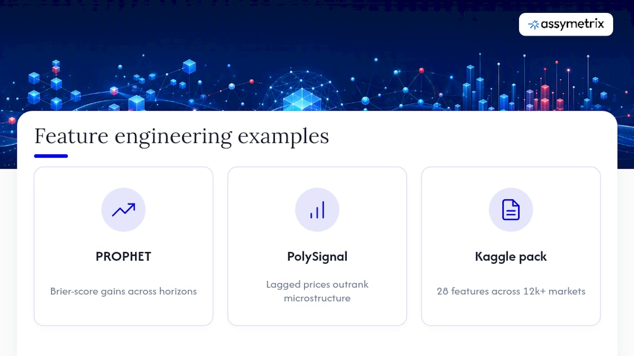
The clearest public demonstration of multi-modal feature engineering paying off comes from the PROPHET ensemble framework, which fused temporal price dynamics with microstructure and contextual signals and reported measurable Brier-score gains over single-signal baselines, with the improvement holding across multiple forecast horizons rather than a single lucky window. That multi-horizon robustness check is the part worth replicating even if the exact architecture isn’t.
On the feature-importance side, the production pipeline behind PolySignal found price_lag7 outranking shorter lags and most microstructure features when identifying mispriced Polymarket contracts, a concrete, reproducible result rather than a general claim about lagged prices mattering. Anyone building a first feature set can validate this against their own data before assuming it generalizes to a different market category.
At the dataset level, the Kaggle engineered-features release packaging 28 pre-computed features across more than 12,000 markets shows what a mature feature table looks like structurally: price dynamics, volume ratios, microstructure, and time-decay columns sitting side by side, ready for a training loop without a separate normalization pass. Each of these examples shares a trait worth noting: none of them treat a single feature category as sufficient on its own. The gains come from combining categories that capture different information, price history, order flow, and time structure, rather than optimizing one family in isolation.
Priorities and Pitfalls Worth Repeating
Reproducible timestamps and canonical IDs matter more than model architecture. Decouple signal generation from execution before you decouple anything else. Watch for leakage, for models overfitting to low-liquidity noise, and for underestimating execution friction. Measure real progress in calibrated probability gains and realized PnL after honest costs, not backtest Sharpe ratios.
— Dean
Get Unified Cross-Venue Data Without Building Three Integrations
Every pipeline described above assumes you can get clean trades, orderbook depth, OHLCV, and wallet activity from Polymarket, Kalshi, and Limitless without reconciling three schemas yourself. That reconciliation work is what the Assymetrix Data API removes, built on roughly 1.5 terabytes of historical data spanning close to a billion rows of trading activity across all three venues.

If you’re starting from the recipes in this guide, pull the minimal feature set (price_lag7, bid_ask_imbalance, cross_venue_spread, smart_money_entry_flag, and the rest) directly against a normalized feed rather than writing separate collectors per venue. The API ships raw trades, orderbook snapshots, and wallet fills alongside pre-computed feature snapshots for teams who want to skip the pipeline-building step entirely and go straight to model training. Pricing details are available on request through the Data API page. Start there, pull a reproducible historical snapshot for your backtest window, and run the walk-forward validation checklist above before committing capital to any signal.
Sources
FAQ
What Is the Most Predictive Single Feature for Prediction Markets?
Seven-day price lag (price_lag7) ranked as the top predictor in a reproduced feature-importance study on Polymarket contracts, outperforming shorter lags and most microstructure features. It shouldn’t be used alone, but it’s a strong first feature to validate against your own data.
Why Do Cross-Venue Features Outperform Single-Venue Features?
A single venue’s price reflects only its own order flow and liquidity, not the market’s full view of an event. Cross-venue spreads and synthetic Dutch-book calculations expose fragmentation between venues pricing the same event differently, which single-venue models can’t see at all.
How Do I Avoid Feature Leakage in Prediction-Market Models?
Compute every feature using only data that existed at that exact timestamp, and validate with walk-forward, time-aware splits rather than random k-fold cross-validation. Leakage is widely considered the most common failure mode in this kind of modeling, and it’s almost always caught by strict timestamp hygiene.
Does Assymetrix Provide Wallet and Smart Money Data?
Yes. The Assymetrix Data API includes wallet fills, holder snapshots, and Smart Money tracking alongside trades, orderbook snapshots, and OHLCV across Polymarket, Kalshi, and Limitless. Current pricing for the API is available on the Assymetrix site.
What Metric Should I Use to Validate a Prediction-Market Model?
The Brier score is the standard calibration metric, paired with calibration plots comparing predicted probability buckets to realized outcome frequency. A multi-modal ensemble approach showed measurable Brier-score improvement over baseline models with robustness holding across multiple forecast horizons, which is a useful benchmark for judging your own results.
Feature Engineering for Devs: 9 Predictors for Prediction Markets
Six feature families consistently separate profitable prediction-market models from noise: price lag and momentum, orderbook microstructure, volume anomalies, time-to-expiry decay, Smart Money wallet entries, and cross-venue spreads. None of them work in isolation, and none of them work well on single-venue data. Cross-venue, timestamped, normalized data is what turns these signals into a tradable edge rather than a backtest artifact, and that is the piece most home-grown pipelines get wrong. A Data API exists that provides developers with a unified feed of trades, orderbook snapshots, OHLCV, and wallet activity across Polymarket, Kalshi, and Limitless without requiring three separate integrations.
TL;DR:
The most predictive features include seven-day price lag and cross-venue spreads, which outperform single-venue signals by exposing market fragmentation.
Cross-venue, timestamped, normalized data significantly enhances model accuracy, and a unified API simplifies data collection from Polymarket, Kalshi, and Limitless.
Preventing feature leakage requires strict timestamp discipline and walk-forward validation, as using pre-resolution data can create misleading backtest results.
A small, well-chosen feature set—such as lagged prices, bid-ask imbalance, and wallet activity—combined with multiple temporal cadences yields reliable initial models.
Proper feature engineering emphasizes reproducibility, interpretability, and realistic validation, with the Brier score commonly used to measure calibration and forecasting accuracy.
AssymetrixBuild With Unified Market DataAssymetrix gives developers and AI agents unified prediction market data across Polymarket, Kalshi, and Limitless through one integration.Explore Assymetrix
Table of Contents
What Feature Categories Actually Predict Resolution Outcomes?
How Do You Engineer Features From Raw Trade and Orderbook Data?
Why Separate the Feature Engine From the Signal Engine?
How Should You Validate Prediction-Market Signals?
How Does a Unified Data API Speed Up Feature Engineering?
What’s a Good Starter Feature Set for a First Model?
Feature Selection and Dimensionality Reduction for Prediction-Market Models
How Do You Interpret Feature Importance in These Models?
What Are the Most Common Feature Engineering Mistakes?
What Does Successful Feature Engineering Look Like in Practice?
Priorities and Pitfalls Worth Repeating
Get Unified Cross-Venue Data Without Building Three Integrations
Sources
What Feature Categories Actually Predict Resolution Outcomes?
Most prediction-market models fail not because of weak algorithms but because of shallow feature sets pulled from a single venue’s price history. The categories below carry the actual signal.
Price dynamics. Lagged prices at 1, 3, and 7 periods, momentum (rate of change), acceleration (second derivative of momentum), and distance from 0.5 all matter, but not equally. A reproduced feature-importance study on a production Polymarket pipeline found that price_lag7 ranked as the single most important predictor for identifying mispriced contracts, ahead of shorter lags and most microstructure inputs.
Microstructure and liquidity. Bid-ask spread, effective spread, order-book depth, and bid-ask imbalance function as proxies for informed trading and execution risk. A wide spread on a thinly traded contract tells you the last print is unreliable; a persistent one-sided imbalance often precedes a directional move before the mid-price adjusts.
Volume dynamics. Volume spikes, volume moving-average ratios, and volume acceleration flag new information hitting the market, often before price fully reflects it.
Temporal features. Hours-to-expiry, time-decay curves, and calendar effects around scheduled resolution events (elections, earnings, Fed meetings) shape how variance behaves as a market approaches settlement. Deadline-resolution structure changes the statistics of the underlying process itself, which is why structural volatility models built around deadline dynamics tend to outperform standard GARCH approaches on these instruments.
Smart Money and trader features. Wallet-entry flags, concentration of top-decile wallets in a market, and trader-skill scores built from historical resolution accuracy.
Cross-venue features. Matched-event price spreads and synthetic Dutch-book cost, which expose fragmentation between venues pricing the same real-world event differently.
A public dataset covering more than 12,000 Polymarket markets and 28 pre-computed features spanning price, volume, and microstructure categories is a useful reference point for what a mature feature table looks like in practice.
How Do You Engineer Features From Raw Trade and Orderbook Data?
Turning raw trades, orderbook snapshots, OHLCV bars, and wallet events into model-ready features follows a repeatable sequence.
Canonicalize first. Map every venue-specific market ID to a single canonical
market_id, normalize price units (Polymarket and Kalshi don’t express probability the same way), and align every timestamp to UTC before anything else happens.Pick your cadence deliberately. Trade-level granularity captures every microstructure shift but multiplies storage and compute; 1-minute snapshots suit latency-sensitive signals; 15-minute or daily snapshots suit slower research loops. Most teams run two parallel cadences rather than one.
Write formulas as explicit, testable functions, not ad hoc notebook cells:
price_lag7 = price[t-7],price_velocity = (price[t] - price[t-k]) / k,bid_ask_imbalance = (bid_size - ask_size) / (bid_size + ask_size),liquidity_pressure = spread * volume,hours_to_expiry = (resolution_ts - t) / 3600,smart_money_entry_flag = 1 if top_wallet_trade_size > threshold else 0.Handle missing data explicitly. Forward-fill price series across low-liquidity gaps, use neutral (0.5) imputation for probability fields when no trade occurred, and always add a boolean mask column so the model can distinguish “no signal” from “zero signal.”
Store features as time-indexed, versioned tables, ideally as parquet snapshots keyed by
market_idandfeature_timestamp, so backtests are reproducible months later.
Persistent snapshotting matters more than it sounds. Polymarket’s public endpoints don’t guarantee historical completeness for older markets, so a collector that only polls live data will silently lose the tail history you need for walk-forward testing.
Pro Tip: Compute every feature as of its own timestamp and store that timestamp alongside it. If you can’t reconstruct exactly what your model would have seen at 2:14 PM on a given day, you can’t trust your backtest.
Why Separate the Feature Engine From the Signal Engine?
A clean architecture keeps research honest and execution flexible: collector → normalizer → feature engine → signal engine → risk filter → execution. Each stage does one job and hands off a well-defined object to the next.
The signal engine should emit a structured, timestamped object rather than a raw prediction, as emphasized by the importance of real-time betting analytics for bettors and analysts. A workable schema includes:
token_id,direction,score,confidencefair_valueversusmarket_price(the actual mispricing estimate)reason(which features drove the call, for debugging and audit)signal_time,market_state,execution_price,outcome(filled in after resolution, for backtesting)
This structure exists because an explainable, timestamped signal object makes backtests reproducible and lets multiple execution strategies consume the same signal without re-running the feature pipeline. Latency matters here too: WebSocket feeds beat polling for markets where prices move on news, and every signal consumer needs a stale-state guard that discards signals built on data older than a defined threshold. Separating research from execution also means you never accidentally place an order while testing a feature change, a real failure mode when the two are entangled in one script.
How Should You Validate Prediction-Market Signals?
A model that looks good on a naive backtest and fails live almost always has a leakage problem. Validation discipline is not optional here.
Walk-forward validation with time-aware splits, never random k-fold, since random splits let future information leak into training.
Strict timestamp hygiene: every feature must be computed using only data that existed at that exact moment. This single rule catches most silent leakage bugs.
Calibration metrics, primarily the Brier score, plus calibration plots comparing predicted probability buckets against realized outcome frequency.
Trade realism: simulate spreads, slippage, and partial-fill probability, and deduct trading fees before reporting any PnL number.
Statistical controls: block bootstrap for confidence intervals on time-series returns, and a deflated Sharpe ratio when you’ve tested more than a handful of feature combinations, since repeated testing inflates apparent performance.
A multi-modal ensemble fusing temporal price dynamics with microstructure signals showed a measurable Brier-score improvement over single-signal baselines, with robustness holding across multiple forecast horizons rather than one lucky window. That kind of multi-horizon check is worth running on your own pipeline before trusting any single backtest period.
How Does a Unified Data API Speed Up Feature Engineering?
The single biggest time cost in prediction-market ML work isn’t modeling. It’s reconciling three inconsistent data schemas before a single feature can be computed.
A unified feed needs to deliver: trade records (timestamp, price, size), full orderbook snapshots with bid and ask depth, OHLCV candles at multiple cadences, wallet fills and holder snapshots for Smart Money tracking, and market metadata including resolution rules and expiry timestamps.
What that removes from your workload:
Canonical ID mapping across Polymarket, Kalshi, and Limitless so the same real-world event isn’t three unrelated database rows.
Price-unit conversion between venues that express probability differently.
Timezone alignment across feeds with different default clocks.
Matched-event grouping, the prerequisite for any cross-venue spread or synthetic Dutch-book calculation.
The practical payoff shows up fastest in cross-venue spread computation and Smart Money tracking, where reconciling raw feeds by hand can eat days per venue pair. Assymetrix’s venue-specific Polymarket resources cover the on-chain quirks worth knowing before you build against that feed directly, and the same normalization logic extends to backtests that need genuine historical completeness rather than whatever the last 30 days of a public endpoint happen to retain.
What’s a Good Starter Feature Set for a First Model?
Nine features, three cadences, and two model families cover most first iterations reasonably well.
Core recipe:
price_lag7,price_velocity_24h,mid_price,spread,bid_ask_imbalance,log_volume_24h,hours_to_expiry,smart_money_entry_flag,cross_venue_spread.Cadences: 1-minute bars for latency-sensitive signals, 15-minute for standard production research, daily and weekly windows for momentum baselines.
Modeling shortcuts: scale all numeric features before training, use gradient-boosted trees as a strong baseline that handles feature interactions natively, and run ElasticNet in parallel for an interpretable comparison point.
Evaluation checklist: Brier score against a naive baseline, calibration plots by probability bucket, simulated PnL after realistic friction, and performance stability across at least two different time horizons.
Pro Tip: Run the ElasticNet baseline even if you plan to ship a tree model. When the linear model captures 80% of the tree model’s accuracy, your edge is coming from a handful of strong features, not complex interactions, and that tells you where to spend your next engineering hour.
Feature Selection and Dimensionality Reduction for Prediction-Market Models
Prediction-market feature sets grow fast once you add lags, ratios, and cross-venue variants of the same base signals, and that growth creates real collinearity problems. price_lag1, price_lag3, and price_lag7 are correlated by construction, and stacking all three plus their velocity derivatives into a tree model can mask which one actually drives predictions.
Start with a correlation filter to drop near-duplicate lag features, keeping the ones with the strongest standalone importance rather than every variant. From there, permutation importance on a held-out time slice tells you which features degrade performance when shuffled, a more honest signal than in-sample importance scores from a single tree ensemble.
Recursive feature elimination works reasonably well for prediction markets because the feature count per market is usually manageable (under 50 in most engineered sets), unlike high-dimensional text or image problems. Principal component analysis is less useful here since it destroys the interpretability that matters for the reason field in your signal schema. If you need dimensionality reduction for a specific reason, like combining multiple wallet-concentration metrics into a single Smart Money composite score, do it deliberately with a named formula rather than an opaque PCA component.
The practical target is a feature set small enough to audit by hand, ten to fifteen features rather than eighty, where every survivor earns its place through out-of-sample importance rather than intuition.
How Do You Interpret Feature Importance in These Models?
Feature importance in a prediction-market model answers a narrower question than most practitioners assume: it tells you which inputs the model leaned on for its historical predictions, not which inputs represent a durable market inefficiency. Those are different claims, and conflating them is how overfit features survive into production.
Tree-based models (gradient boosting, random forests) report importance through split-count or gain metrics natively, but these numbers are biased toward high-cardinality features and can overstate the value of noisy volume ratios. SHAP values give a more reliable per-prediction breakdown and let you check whether a feature’s contribution direction matches intuition, a positive bid_ask_imbalance should push probability toward the imbalanced side, and if it doesn’t, that’s a debugging signal, not a nuance to explain away.
The reason field in a well-built signal schema forces this discipline at the point of generation rather than after the fact. If a signal engine can’t state in plain terms which two or three features drove a given call, that signal isn’t ready to trade regardless of its backtested Brier score. Interpretability here isn’t an academic nicety, it’s what lets you distinguish a feature capturing genuine informed-trading behavior from one that happened to correlate with a handful of favorable outcomes in a limited historical sample.
What Are the Most Common Feature Engineering Mistakes?
Leakage is the mistake that ends careers quietly. It happens most often when a feature is computed using data that technically postdates the timestamp it’s assigned to, a resolution outcome bleeding into a pre-resolution feature, or a rolling window that accidentally includes the current bar instead of stopping at the prior one. The single most common failure mode in prediction-market pipelines is exactly this kind of leakage, which is why strict timestamp discipline and walk-forward validation aren’t optional steps, they’re the whole point of the exercise.
A second recurring trap is overfitting to low-liquidity noise. Markets with a handful of daily trades produce price series that look like signal but are really just the last two traders setting an arbitrary print. Features built on these markets can dominate a backtest’s apparent edge while contributing nothing tradable, since you can’t actually execute size against that liquidity.
Underestimating execution friction ranks close behind.
Finally, treating single-venue price as ground truth is a structural error, not a modeling one. A price on one venue reflects that venue’s order flow and liquidity conditions, not the market’s collective view of the underlying event.
What Does Successful Feature Engineering Look Like in Practice?
The clearest public demonstration of multi-modal feature engineering paying off comes from the PROPHET ensemble framework, which fused temporal price dynamics with microstructure and contextual signals and reported measurable Brier-score gains over single-signal baselines, with the improvement holding across multiple forecast horizons rather than a single lucky window. That multi-horizon robustness check is the part worth replicating even if the exact architecture isn’t.
On the feature-importance side, the production pipeline behind PolySignal found price_lag7 outranking shorter lags and most microstructure features when identifying mispriced Polymarket contracts, a concrete, reproducible result rather than a general claim about lagged prices mattering. Anyone building a first feature set can validate this against their own data before assuming it generalizes to a different market category.
At the dataset level, the Kaggle engineered-features release packaging 28 pre-computed features across more than 12,000 markets shows what a mature feature table looks like structurally: price dynamics, volume ratios, microstructure, and time-decay columns sitting side by side, ready for a training loop without a separate normalization pass. Each of these examples shares a trait worth noting: none of them treat a single feature category as sufficient on its own. The gains come from combining categories that capture different information, price history, order flow, and time structure, rather than optimizing one family in isolation.
Priorities and Pitfalls Worth Repeating
Reproducible timestamps and canonical IDs matter more than model architecture. Decouple signal generation from execution before you decouple anything else. Watch for leakage, for models overfitting to low-liquidity noise, and for underestimating execution friction. Measure real progress in calibrated probability gains and realized PnL after honest costs, not backtest Sharpe ratios.
— Dean
Get Unified Cross-Venue Data Without Building Three Integrations
Every pipeline described above assumes you can get clean trades, orderbook depth, OHLCV, and wallet activity from Polymarket, Kalshi, and Limitless without reconciling three schemas yourself. That reconciliation work is what the Assymetrix Data API removes, built on roughly 1.5 terabytes of historical data spanning close to a billion rows of trading activity across all three venues.
If you’re starting from the recipes in this guide, pull the minimal feature set (price_lag7, bid_ask_imbalance, cross_venue_spread, smart_money_entry_flag, and the rest) directly against a normalized feed rather than writing separate collectors per venue. The API ships raw trades, orderbook snapshots, and wallet fills alongside pre-computed feature snapshots for teams who want to skip the pipeline-building step entirely and go straight to model training. Pricing details are available on request through the Data API page. Start there, pull a reproducible historical snapshot for your backtest window, and run the walk-forward validation checklist above before committing capital to any signal.
Sources
FAQ
What Is the Most Predictive Single Feature for Prediction Markets?
Seven-day price lag (price_lag7) ranked as the top predictor in a reproduced feature-importance study on Polymarket contracts, outperforming shorter lags and most microstructure features. It shouldn’t be used alone, but it’s a strong first feature to validate against your own data.
Why Do Cross-Venue Features Outperform Single-Venue Features?
A single venue’s price reflects only its own order flow and liquidity, not the market’s full view of an event. Cross-venue spreads and synthetic Dutch-book calculations expose fragmentation between venues pricing the same event differently, which single-venue models can’t see at all.
How Do I Avoid Feature Leakage in Prediction-Market Models?
Compute every feature using only data that existed at that exact timestamp, and validate with walk-forward, time-aware splits rather than random k-fold cross-validation. Leakage is widely considered the most common failure mode in this kind of modeling, and it’s almost always caught by strict timestamp hygiene.
Does Assymetrix Provide Wallet and Smart Money Data?
Yes. The Assymetrix Data API includes wallet fills, holder snapshots, and Smart Money tracking alongside trades, orderbook snapshots, and OHLCV across Polymarket, Kalshi, and Limitless. Current pricing for the API is available on the Assymetrix site.
What Metric Should I Use to Validate a Prediction-Market Model?
The Brier score is the standard calibration metric, paired with calibration plots comparing predicted probability buckets to realized outcome frequency. A multi-modal ensemble approach showed measurable Brier-score improvement over baseline models with robustness holding across multiple forecast horizons, which is a useful benchmark for judging your own results.
Other Blog


