How to Feed Prediction Market Data into an AI Trading Agent

TL;DR:

• Prediction markets offer binary, verifiable signals that simplify labeling for AI modeling.

• A normalized Pulse data pipeline with deterministic execution improves strategy robustness and backtesting accuracy.

The core method: normalize venue feeds from Polymarket, Kalshi, and Limitless into a timestamped canonical Pulse record, apply liquidity and quality filters at ingestion, convert validated Pulses into feature vectors for an alpha model, then route deterministic sizing and execution through a separate execution layer with hard risk constraints. That separation, forecast from execution, is where most agent implementations either succeed or break down.

Immediate next steps for engineers:

• Subscribe to the Assymetrix WebSocket feed for unified cross-venue streaming across Polymarket, Kalshi, and Limitless

• Implement a liquidity pre-filter at ingestion: drop markets below your minimum threshold before any downstream processing

• Normalize every incoming payload to a canonical Pulse schema with fields: market_id, venue, mid_price, liquidity, bid_depth, ask_depth, resolution_ts, and ingestion_ts

• Build a feature store that accepts Pulse writes at sub-100ms latency for time-sensitive strategies

• Keep your alpha model’s output to a probability estimate and confidence score; route sizing and risk controls through a deterministic execution layer

• Backtest using archived Pulse replay with walk-forward validation, not in-sample fitting

Assymetrix’s Data API at data.assymetrix.com covers all three major venues through a single integration, backed by extensive historical data spanning a very large number of rows of trading activity.

Table of Contents

• Why prediction markets give AI agents a structural edge

• What data does your AI agent actually need?

• How to architect the data pipeline from ingest to signal API

• How to normalize venue schemas into a canonical Pulse

• Feature engineering and separating your alpha model from execution

• How the execution layer controls order placement and slippage

• How to backtest prediction market strategies without overfitting

• Production concerns: latency, monitoring, security, and cost

• Assymetrix WebSocket integration: Python code that builds a feature vector

• Common failure modes and how to fix them

• Key Takeaways

• The part most teams get wrong

• Assymetrix gives your AI agent a production-ready data foundation

• Useful sources

• FAQ

Why prediction markets give AI agents a structural edge

Prediction markets produce a specific kind of signal that most financial data sources cannot: a crowd-aggregated probability estimate on a binary, verifiable outcome. When an election resolves, a contract settles to $1.00 or $0.00. There is no ambiguity in the label. For supervised learning, that binary resolution eliminates the label-construction problem that plagues equity or macro models, where “correct” outcomes are contested or delayed.

Real-time order book data on Polymarket, Kalshi, and Limitless reflects the aggregated beliefs of active participants updating continuously on new information. Research into the mathematical structure of prediction market pricing shows that prices follow dynamics related to stochastic mirror descent, meaning instantaneous price points are noisy but time-averaged prices converge toward better consensus estimates. That property has a direct engineering implication: your feature pipeline should compute time-weighted averages, not raw ticks, for most model inputs.

Cross-venue confirmation adds a second layer of signal quality. When Polymarket and Kalshi price the same event within a tight spread, that agreement is a stronger signal than either venue alone. Divergence between venues, on the other hand, is itself a tradeable signal and a data quality flag.

Key signal properties for AI agent design:

• Binary, verifiable outcomes reduce label ambiguity for training and calibration

• Real-time pricing reflects fast-updating crowd beliefs, not stale analyst estimates

• Cross-venue confirmation reduces single-venue noise and flags manipulation

• Resolution metadata provides ground-truth labels for model evaluation

• Liquidity metrics gate signal quality: low-liquidity markets are high-noise by default

Assymetrix aggregates all three major venues into a single normalized feed, which means your agent receives cross-venue confirmation signals without building three separate connectors. The AI agents in prediction markets developer guide covers the full automation stack from ingestion to execution.

What data does your AI agent actually need?

The gap between “I have a WebSocket connection” and “my model has usable features” comes down to which fields you capture and at what granularity. Agents need both real-time streams for inference and historical records for training.

Real-time data types:

• Price ticks (best bid, best ask, mid price, last trade price)

• Order book depth snapshots (top N levels, bid/ask quantities)

• Trade stream (size, direction, timestamp, taker wallet)

• Timestamped liquidity metrics (total open interest, 24h volume, spread)

• Fee schedule per venue (affects net EV calculations)

Historical and contextual data types:

• OHLC snapshots at configurable intervals (1m, 5m, 1h)

• Resolution metadata: slug, conditionId, resolution rules, resolution date, settlement value

• Historical settlement records for training label construction

• Wallet activity signals (smart money indicators, large-position tracking)

• Event correlation data across related markets

Canonical ingestion schema:

For production inference, aim for tick-level ingestion with sub-second timestamps. For training, 1-minute OHLC snapshots with full resolution history are sufficient for most event-forecasting models. Wallet activity signals from Smart Money tracking add a high-value feature layer that raw price feeds alone cannot provide.

How to architect the data pipeline from ingest to signal API

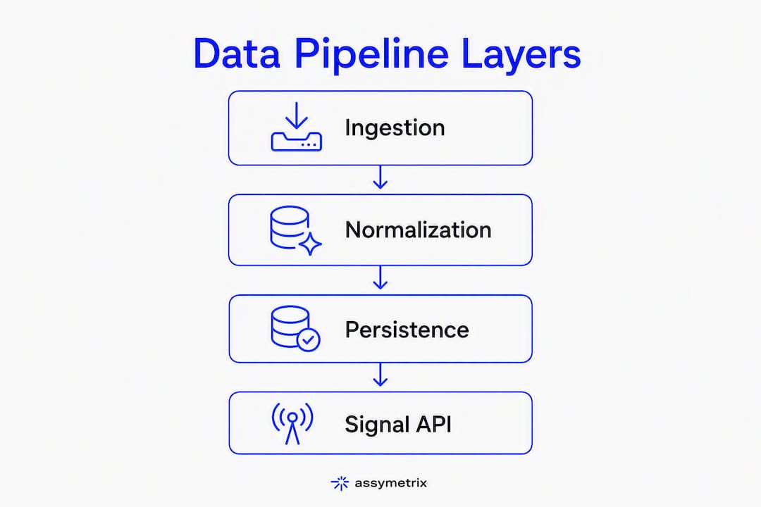
A production-grade prediction market data pipeline has four distinct layers. Conflating them, especially mixing normalization logic with model inference, is the most common architectural mistake in early-stage agent builds.

Layer 1: Ingestion (venue connectors)

Connector workers maintain persistent WebSocket connections to each venue. Each worker deserializes raw payloads, stamps an ingestion_ts, and publishes to a message bus (Kafka works well here). The connector’s only job is reliable delivery; no transformation happens at this layer.

Layer 2: Normalization (Pulse generation)

A normalization worker consumes raw messages from the bus, applies the canonical schema mapping, runs quality checks, and emits validated Pulse records. Liquidity pre-filtering happens here: markets below your minimum liquidity threshold are dropped before any downstream processing. predict-raven’s architecture organizes this as Layer 1 (Research/Pulse), with explicit separation from the decision and execution layers.

Layer 3: Feature store and persistence

Validated Pulses write to both a time-series store (for historical replay and backtest) and an online feature store (for low-latency inference reads). The online store must support sub-100ms reads for time-sensitive strategies.

Layer 4: Signal API and decision runtime

The alpha model reads features from the online store via a synchronous signal API, emits a probability estimate and confidence score, and hands off to the execution layer. The execution layer applies deterministic risk rules before any order instruction reaches a venue connector.

Live trade dataflow:

• Event published on Polymarket → connector worker receives WebSocket message

• Raw payload published to Kafka topic raw_pulses

• Normalization worker reads, validates, applies liquidity filter, emits canonical Pulse

• Pulse written to online feature store and time-series archive

• Signal API reads latest features, calls alpha model, receives {p: 0.72, confidence: 0.81}

• Execution layer applies Kelly sizing, checks exposure caps, emits order instruction

• Order instruction routed to venue connector for placement

Pro Tip: Implement the liquidity pre-filter at the normalization layer, not inside the model. Markets below your threshold should never reach the feature store. Filtering downstream wastes compute and risks noisy records contaminating feature distributions.

How to normalize venue schemas into a canonical Pulse

Polymarket, Kalshi, and Limitless each use different field names, price representations, and order book formats. Your normalization layer must absorb those differences and emit a consistent Pulse that downstream components never need to inspect for venue origin.

Canonical Pulse fields:

market_id, venue, side, mid_price, liquidity, bid_depth, ask_depth, fees, resolution_ts, last_trade_ts, ingestion_ts, raw_event_hash

Vendor field mapping:

Data quality checklist:

• Schema validation: all required fields present and correctly typed

• Timestamp monotonicity: reject any Pulse with ingestion_ts earlier than the previous record for the same market_id

• Duplicate suppression: compare raw_event_hash against a rolling dedup window

• Stale-data rule: treat any Pulse with last_trade_ts more than 120 minutes old as a risk state; flag it and exclude from active inference

• Payload hashing: SHA-256 the raw venue payload before transformation for audit trail integrity

Prediction market pricing research confirms that instantaneous price points are noisy and that time-averaging improves consensus estimates. Apply a time-weighted average price (TWAP) over a configurable window (typically 5–15 minutes) as your primary mid_price feature rather than the raw last-trade price.

Pro Tip: Compute TWAP over a short rolling window before writing to the feature store. A single large trade can spike the raw mid_price by several percentage points on low-liquidity markets. TWAP smooths that transient noise and produces a more stable consensus estimate for your model.

Feature engineering and separating your alpha model from execution

The feature set for a prediction market agent differs from equity or crypto feature sets in one important way: resolution timing is a first-class feature. A market pricing at 0.65 with 30 days to resolution has very different capital efficiency than the same price with 6 hours remaining.

Recommended feature set:

• price_momentum_1h, price_momentum_24h: rolling price change over fixed windows

• liquidity_adjusted_spread: (ask - bid) / mid_price, weighted by liquidity score

• order_book_imbalance: (bid_depth - ask_depth) / (bid_depth + ask_depth)

• time_to_resolution_hours: (resolution_ts - now) / 3600

• monthly_return_score: edge / months_to_resolution (normalizes for capital efficiency)

• smart_money_flow: net wallet flow from high-skill traders over rolling window

• cross_venue_divergence: absolute difference in mid_price across venues for same event

• smoothed_implied_prob: TWAP-based probability estimate

• model_confidence: calibration score from the alpha model’s last inference

Model responsibility map:

The alpha model’s job is probability estimation, nothing else; for a proven example of modular agent design and leaderboard-style performance reporting, see TradeAiFi™ — AI Trading Platform leaderboard. Research on the Raven-Agent architecture shows that a deterministic, composable trading layer that separates selection, sizing via fractional Kelly, and risk control produces better risk-adjusted returns than end-to-end learned sizing. The execution model enforces sizing rules; the alpha model never touches position sizing directly.

Pro Tip: Keep sizing deterministic. Use fractional Kelly or fixed-stake rules, and keep sizing logic entirely outside the model prompt or inference call. Optiver’s analysis of AI trading models identifies execution precision as the binding constraint: models often understand expected value but fail to execute with the necessary sizing discipline. A deterministic sizing layer eliminates that failure mode.

How the execution layer controls order placement and slippage

The execution layer is not a model. It is a deterministic policy engine with hard constraints that no learned component can override. This distinction matters for auditability and for preventing catastrophic failures when a model produces an overconfident or hallucinated output.

Execution rules (enforce all of these):

• Per-trade notional cap: maximum dollar exposure per single order

• Aggregate exposure cap: total open notional across all positions

• Per-event correlation cap: limit exposure to correlated events (same underlying)

• Position-level stop loss: close position if mark-to-market loss exceeds threshold

• Portfolio-level drawdown halt: suspend all trading if portfolio drawdown exceeds limit

• Stale-Pulse rejection: refuse any order instruction based on a Pulse flagged as stale

Order placement patterns:

Use market Fill-or-Kill (FOK) orders when speed matters and the spread is acceptable relative to your EV estimate. Use limit orders when you can afford to wait and the spread cost would materially reduce EV. On Polymarket’s CLOB API, limit orders post to the order book and can be canceled; FOK orders execute immediately or reject. For Kalshi, the REST API supports both market and limit order types with explicit fill semantics.

Practitioners recommend keeping hard risk constraints external to any learned policy. If you use reinforcement learning for execution timing or order slicing, the RL policy should operate within a constrained action space where the deterministic safety checks cannot be bypassed. The RL agent learns when and how much to slice; it never learns to override the exposure cap.

Pro Tip: Test execution policies in a high-fidelity simulator that injects realistic market impact before going live. Slippage assumptions that look fine on historical fills often break down when your agent is the marginal liquidity taker on a thin order book.

How to backtest prediction market strategies without overfitting

Backtesting prediction market agents is harder than it looks. The two most common failure modes are look-ahead bias from centered rolling windows and overfitting to transient price spikes that never recur.

Backtest checklist:

1. Use archived Pulse replay with original timestamps preserved, not reconstructed prices

2. Apply walk-forward validation: train on period T, validate on T+1, never the reverse

3. Enforce a warmup period before any model inference to prevent centered-window leakage

4. Audit every feature for target leakage: no feature should contain information from after the prediction timestamp

5. Use full archived order book snapshots when available for credible counterfactual fill modeling

6. Separate in-sample parameter tuning from out-of-sample performance reporting

AgentQuant’s tooling provides a WarmupEnforcer and procedures to detect centered rolling windows and global normalization leaks, both of which are common in time-series ML pipelines. Apply these checks before any performance number is reported.

Evaluation metrics:

• Brier score: measures probability calibration; lower is better (0.0 = perfect)

• ROC/AUC: classifier-style detection of correct directional calls

• Edge hit rate: fraction of trades where realized outcome matched predicted direction

• Realized EV per trade: (p_predicted * payout) - cost, averaged across all trades

• Sharpe ratio: risk-adjusted return over the backtest window

• Hit rate vs. EV tradeoff: high hit rate with low EV is worse than moderate hit rate with strong EV

Assymetrix’s backtesting guide covers high-fidelity replay using the historical archive. The nearly one billion rows of trading activity in the Assymetrix dataset provide enough depth for statistically meaningful walk-forward validation across multiple event categories.

Production concerns: latency, monitoring, security, and cost

Latency targets:

For strategies that require fast reaction to price updates, target sub-100ms from WebSocket message receipt to feature store write. For slower event-forecasting strategies where resolution is days or weeks away, batch ingestion windows of 1–5 minutes are acceptable and significantly reduce infrastructure cost.

Monitoring checklist:

• Pulse freshness: alert if no new Pulse for a given market_id within expected interval

• Queue backlog size: Kafka consumer lag above threshold indicates ingestion bottleneck

• Data-drop rate: percentage of raw messages that fail schema validation

• Feature distribution drift: monitor mean and variance of key features against baseline

• Model calibration drift: track Brier score on resolved markets over rolling window

• End-to-end P&L vs. expected EV: persistent divergence signals execution or data quality issues

Security and operational controls:

• Store execution wallet keys in a secrets manager (AWS Secrets Manager or HashiCorp Vault), never in environment variables or code

• Segregate paper trading and live trading environments at the network level

• Run preflight checks before each session: verify wallet address, confirm available collateral, test venue API connectivity

• Implement a kill switch that halts all order submission and cancels open orders within one API call

• Log every order instruction with the Pulse hash that triggered it for full audit trail

Cost guidance:

Streaming WebSocket connections are cheap per message but require persistent compute. For high-frequency ingestion across three venues, a dedicated connector process per venue is more reliable than a multiplexed single connection. Cold storage for archived Pulses costs a fraction of hot storage; keep only the last 30 days in hot storage and archive the rest. Backtest compute is the largest variable cost: precompute feature baselines from bulk exports rather than recomputing from raw ticks on every backtest run.

Pro Tip: Optimal market making in prediction markets depends on inventory, time to resolution, and liquidity in ways that differ from classical settings, as stochastic control research shows. If your agent provides liquidity rather than taking it, your latency requirements and quoting strategy need to account for time-to-resolution explicitly, not just spread.

Assymetrix WebSocket integration: Python code that builds a feature vector

The Assymetrix Data API provides a unified WebSocket feed that delivers normalized Pulse messages across Polymarket, Kalshi, and Limitless through a single connection. You do not need separate connectors per venue.

Auth and connection notes:

• Authenticate via API key passed as a query parameter or header on the WebSocket handshake

• Implement exponential backoff reconnection: start at 1 second, cap at 60 seconds, reset on successful message receipt

• Subscribe to specific market slugs or to a full venue stream depending on your strategy scope

WebSocket URL pattern:

wss://data.assymetrix.com/v1/stream?api_key=YOUR_KEY&venues=polymarket,kalshi,limitless

wss://data.assymetrix.com/v1/stream?api_key=YOUR_KEY&venues=polymarket,kalshi,limitless

REST snapshot endpoint:

GET https://data.assymetrix.com/v1/markets/{market_id}/pulse?limit=100

GET https://data.assymetrix.com/v1/markets/{market_id}/pulse?limit=100

Python integration example:

import asyncio
import json
import time
import os
from collections import deque
import websockets

API_KEY = os.environ["ASSYMETRIX_API_KEY"]
WS_URL = f"wss://data.assymetrix.com/v1/stream?api_key={API_KEY}&venues=polymarket,kalshi,limitless"

LIQUIDITY_MIN = 0.10        # Drop markets below this normalized liquidity score
STALE_THRESHOLD_S = 7200    # 120 minutes in seconds
TWAP_WINDOW_S = 300         # 5-minute TWAP window

# Rolling price buffer per market_id for TWAP computation
price_buffers: dict[str, deque] = {}

def compute_feature_vector(pulse: dict) -> dict | None:
    """Convert a validated Pulse record into a feature vector."""
    market_id = pulse["market_id"]
    now = int(time.time())

    # Staleness check
    last_trade_age = now - pulse.get("last_trade_ts", 0)
    if last_trade_age > STALE_THRESHOLD_S:
        return None  # Stale pulse; exclude from inference

    # Liquidity filter
    if pulse.get("liquidity", 0) < LIQUIDITY_MIN:
        return None  # Below threshold; drop before feature computation

    # TWAP computation
    if market_id not in price_buffers:
        price_buffers[market_id] = deque()
    buf = price_buffers[market_id]
    buf.append((now, pulse["mid_price"]))
    # Evict entries outside the TWAP window
    while buf and (now - buf[0][0]) > TWAP_WINDOW_S:
        buf.popleft()
    twap = sum(p for _, p in buf) / len(buf) if buf else pulse["mid_price"]

    # Order book imbalance
    bid_d = pulse.get("bid_depth", 0)
    ask_d = pulse.get("ask_depth", 0)
    total_depth = bid_d + ask_d
    ob_imbalance = (bid_d - ask_d) / total_depth if total_depth > 0 else 0.0

    # Time to resolution (hours)
    resolution_ts = pulse.get("resolution_ts", 0)
    time_to_res_h = max((resolution_ts - now) / 3600, 0)

    return {
        "market_id": market_id,
        "venue": pulse["venue"],
        "mid_price": pulse["mid_price"],
        "twap_5m": round(twap, 6),
        "order_book_imbalance": round(ob_imbalance, 4),
        "liquidity_score": pulse["liquidity"],
        "time_to_resolution_h": round(time_to_res_h, 2),
        "feature_ts": now,
    }

async def push_to_decision_queue(feature_vector: dict):
    """Placeholder: replace with your online feature store write or message bus publish."""
    print(json.dumps(feature_vector))

async def stream_pulses():
    backoff = 1
    while True:
        try:
            async with websockets.connect(WS_URL) as ws:
                backoff = 1  # Reset on successful connection
                async for raw_msg in ws:
                    pulse = json.loads(raw_msg)
                    fv = compute_feature_vector(pulse)
                    if fv:
                        await push_to_decision_queue(fv)
        except (websockets.ConnectionClosed, OSError) as e:
            print(f"Connection error: {e}. Reconnecting in {backoff}s.")
            await asyncio.sleep(backoff)
            backoff = min(backoff * 2, 60)

if __name__ == "__main__":
    asyncio.run(stream_pulses())

import asyncio
import json
import time
import os
from collections import deque
import websockets

API_KEY = os.environ["ASSYMETRIX_API_KEY"]
WS_URL = f"wss://data.assymetrix.com/v1/stream?api_key={API_KEY}&venues=polymarket,kalshi,limitless"

LIQUIDITY_MIN = 0.10        # Drop markets below this normalized liquidity score
STALE_THRESHOLD_S = 7200    # 120 minutes in seconds
TWAP_WINDOW_S = 300         # 5-minute TWAP window

# Rolling price buffer per market_id for TWAP computation
price_buffers: dict[str, deque] = {}

def compute_feature_vector(pulse: dict) -> dict | None:
    """Convert a validated Pulse record into a feature vector."""
    market_id = pulse["market_id"]
    now = int(time.time())

    # Staleness check
    last_trade_age = now - pulse.get("last_trade_ts", 0)
    if last_trade_age > STALE_THRESHOLD_S:
        return None  # Stale pulse; exclude from inference

    # Liquidity filter
    if pulse.get("liquidity", 0) < LIQUIDITY_MIN:
        return None  # Below threshold; drop before feature computation

    # TWAP computation
    if market_id not in price_buffers:
        price_buffers[market_id] = deque()
    buf = price_buffers[market_id]
    buf.append((now, pulse["mid_price"]))
    # Evict entries outside the TWAP window
    while buf and (now - buf[0][0]) > TWAP_WINDOW_S:
        buf.popleft()
    twap = sum(p for _, p in buf) / len(buf) if buf else pulse["mid_price"]

    # Order book imbalance
    bid_d = pulse.get("bid_depth", 0)
    ask_d = pulse.get("ask_depth", 0)
    total_depth = bid_d + ask_d
    ob_imbalance = (bid_d - ask_d) / total_depth if total_depth > 0 else 0.0

    # Time to resolution (hours)
    resolution_ts = pulse.get("resolution_ts", 0)
    time_to_res_h = max((resolution_ts - now) / 3600, 0)

    return {
        "market_id": market_id,
        "venue": pulse["venue"],
        "mid_price": pulse["mid_price"],
        "twap_5m": round(twap, 6),
        "order_book_imbalance": round(ob_imbalance, 4),
        "liquidity_score": pulse["liquidity"],
        "time_to_resolution_h": round(time_to_res_h, 2),
        "feature_ts": now,
    }

async def push_to_decision_queue(feature_vector: dict):
    """Placeholder: replace with your online feature store write or message bus publish."""
    print(json.dumps(feature_vector))

async def stream_pulses():
    backoff = 1
    while True:
        try:
            async with websockets.connect(WS_URL) as ws:
                backoff = 1  # Reset on successful connection
                async for raw_msg in ws:
                    pulse = json.loads(raw_msg)
                    fv = compute_feature_vector(pulse)
                    if fv:
                        await push_to_decision_queue(fv)
        except (websockets.ConnectionClosed, OSError) as e:
            print(f"Connection error: {e}. Reconnecting in {backoff}s.")
            await asyncio.sleep(backoff)
            backoff = min(backoff * 2, 60)

if __name__ == "__main__":
    asyncio.run(stream_pulses())

Code assumptions:

• ASSYMETRIX_API_KEY must be set as an environment variable

• Pulse messages contain at minimum: market_id, venue, mid_price, liquidity, bid_depth, ask_depth, last_trade_ts, resolution_ts

• push_to_decision_queue is a stub; replace with your Redis, Kafka, or feature store write

• Polymarket-specific metadata (e.g., conditionId) and Kalshi-specific fields (e.g., ticker) arrive in the Pulse’s metadata sub-object and can be extracted for venue-specific model variants

Pro Tip: Use Assymetrix’s historical bulk export to precompute normalization baselines (mean, standard deviation, liquidity percentiles) before going live. Feature scaling calibrated on live data only introduces look-ahead bias into your production pipeline.

The Assymetrix real-time API guide covers venue-specific field idiosyncrasies for Kalshi and Polymarket connectors in detail.

Common failure modes and how to fix them

Most prediction market agent failures are not model failures. They are data pipeline failures that corrupt the inputs before the model ever sees them.

Failure modes and mitigations:

• Low-liquidity noise: thin markets produce erratic price swings that look like signals. Mitigation: enforce a minimum liquidity threshold at the normalization layer; never let sub-threshold markets reach the feature store.

• Wash trading or manipulation: coordinated trades can move prices on low-volume markets. Mitigation: apply wallet-flow heuristics to detect concentrated trading from a small number of addresses; cross-venue confirmation reduces the impact of single-venue manipulation.

• Stale or missing resolution metadata: a market without a clear resolution date or rules cannot produce valid time_to_resolution features. Mitigation: require resolution_ts and resolution_rules as mandatory Pulse fields; reject records missing either.

• Look-ahead bias in backtests: centered rolling windows and global normalization are the two most common leakage vectors. Mitigation: use WarmupEnforcer from AgentQuant and walk-forward validation.

• Overfitting to transient price spikes: a model trained on raw ticks will learn spike patterns that do not generalize. Mitigation: use TWAP features rather than raw last-trade prices; apply minimum observation counts before including a market in training data.

Pro Tip: Randomize execution timing and order slicing on low-liquidity markets. Predictable order patterns signal your flow to other participants, who can front-run or fade your positions. Small random delays of 0.5–3 seconds and variable order sizes reduce your footprint significantly.

Key Takeaways

Feeding prediction market data into an AI trading agent requires a normalized Pulse pipeline, strict separation of alpha and execution models, and rigorous walk-forward backtesting to avoid overfitting to noisy price history.

The part most teams get wrong

The conventional framing of prediction market agent development focuses almost entirely on the forecasting model: which architecture, which features, which training objective. That focus is misplaced. The forecasting model is rarely the binding constraint.

What actually breaks production agents is the execution layer, or more precisely, the absence of one. Teams build a capable probability estimator, then route its output directly to an order placement call with no deterministic sizing, no exposure caps, and no stale-data checks. The model produces a confident estimate on a market that last traded three hours ago. The order goes through. The position is illiquid. The loss is real.

The Raven-Agent research makes this concrete: the only architecture that produced positive risk-adjusted returns in controlled replay was the one with an explicit, deterministic trading layer separating selection, sizing, and risk control. Not the most sophisticated forecaster. The most disciplined executor.

The second thing teams underestimate is the cost of multi-venue integration. Building and maintaining three separate connectors for Polymarket, Kalshi, and Limitless, each with different schemas, authentication patterns, and rate limits, consumes engineering time that should go toward model development and backtesting. A unified feed that normalizes at the source changes the economics of the whole project.

Start with the Pulse schema. Get the execution layer deterministic before you tune the model. Run walk-forward validation before you report any performance number. Those three decisions, made early, determine whether the project ships or stalls.

Assymetrix gives your AI agent a production-ready data foundation

Cross-venue prediction market data integration is the first hard problem every agent developer hits. Polymarket, Kalshi, and Limitless each have different schemas, authentication flows, and rate limits. Building three connectors and keeping them synchronized is weeks of engineering before you write a single model feature.

Assymetrix solves that at the infrastructure layer. The Data API at data.assymetrix.com delivers a unified, normalized Pulse stream across all three venues through a single WebSocket connection, with REST endpoints for snapshots and bulk historical export. The historical archive covers nearly one billion rows of trading activity, giving your backtest engine the depth it needs for credible walk-forward validation. On top of the raw feed, Assymetrix surfaces Smart Money wallet tracking, cross-venue arbitrage signals, and Trader Skill Scores as ready-to-use features your alpha model can consume directly.

For developers evaluating data quality before committing to a subscription, the prediction market accuracy data guide provides a detailed breakdown of resolution accuracy and signal reliability across venues. The AI agents developer guide walks through the full integration stack. Start with a free API key at data.assymetrix.com and run the Python WebSocket example against live data today.

Useful sources

Primary references and further reading for engineers building prediction market data pipelines:

• predict-raven (Alchemist-X/predict-raven): reference implementation of the Pulse concept, three-layer architecture, and runtime logs

• Beyond Forecasting: The Belief-to-Trade Layer in Prediction-Market Agents: Raven-Agent paper on deterministic trading layers and fractional Kelly sizing

• AgentQuant (OnePunchMonk/AgentQuant): tooling for look-ahead bias detection, WarmupEnforcer, and walk-forward validation

• Markets as ML (marketsml): formal connection between prediction market pricing and no-regret learning algorithms

• Optimal Market Making in Prediction Markets: stochastic control framework for latency-aware quoting

• Where AI trading models work (and where they still fall short): Optiver’s analysis of execution precision as the binding constraint

• Assymetrix Data API documentation: WebSocket and REST reference for the unified cross-venue feed

Recommended next steps: run the Python WebSocket example locally against the Assymetrix live feed, then use the bulk historical export to replay archived Pulses for your first walk-forward backtest.

FAQ

Can AI agents reliably predict outcomes in prediction markets?

AI agents can produce well-calibrated probability estimates on binary prediction market outcomes, but prediction is not the binding constraint. Research shows that execution precision, specifically sizing discipline and market impact modeling, is where most agents underperform.

What is the best data source for an AI trading agent on prediction markets?

A unified, normalized feed that covers multiple venues simultaneously produces more reliable signals than any single-venue connection. Assymetrix aggregates Polymarket, Kalshi, and Limitless into a single normalized Pulse stream with nearly one billion rows of historical data for training and backtest.

How do you avoid look-ahead bias when backtesting prediction market strategies?

Use archived Pulse replay with original timestamps preserved, apply walk-forward validation splits, and enforce a warmup period before any model inference. AgentQuant provides a WarmupEnforcer that detects centered rolling windows and global normalization leaks automatically.

Can ChatGPT or a general LLM handle prediction market trading decisions?

LLMs can reason about event probabilities but consistently fail at precise EV-based sizing. Raven-Agent research shows that keeping sizing outside the model prompt and enforcing it through a deterministic execution layer is the approach that produces positive risk-adjusted returns.

What Python libraries do you need to build a prediction market data pipeline?

The core dependencies are websockets for streaming ingestion, asyncio for concurrent connection management, and a time-series store client (Redis, InfluxDB, or similar) for the online feature store. The Assymetrix Python API guide provides SDK examples and client patterns for the full integration stack.