Scale Kelly Betting for Prediction Market Quants: Large N & Data API
Scale Kelly Betting for Prediction Market Quants: Large N & Data API
Scale Kelly Betting for Prediction Market Quants: Large N & Data API
A math-first playbook for quant traders and developers: apply fractional and multivariate Kelly, scale to large N, and integrate cross-venue data APIs.

Scale Kelly Betting for Prediction Market Quants: Large N & Data API
Adaptive fractional Kelly, not full Kelly, is the right default for prediction market sizing: shrink your bet fraction to reflect calibration uncertainty and model fees before you ever post size. Three forces drive this: estimation error in your probability model, platform fees and liquidity limits, and the scaling burden of running many simultaneous positions. The math and a working implementation checklist follow below.
TL;DR:
Fractional Kelly sizing, such as quarter or half Kelly, reduces drawdowns and accounts for probability estimation errors, fees, and liquidity limits.
Adaptive Kelly strategies incorporate confidence levels, shrinking bets when model calibration is unstable or data is sparse, to avoid overbetting.
Including platform fees in the effective price and considering favorite-longshot biases minimizes overestimation of edge and false signals.
Jointly optimizing Kelly across many correlated positions requires correlation discounts or groupings to prevent overexposure and underestimated risk.
Reliable backtesting and real-time calibration monitoring are crucial to prevent overbetting due to outdated fee assumptions, biased models, or correlation misjudgments.
Assymetrixassymetrix.comBuild Kelly Strategies On Unified DataAccess cross venue prediction market data, Smart Money signals, and historical coverage through one integration for research and trading tools.Explore Assymetrix data
Table of Contents
Mathematical foundations of Kelly for binary contracts
Kelly as information-theoretic and Bayesian model evaluation
Fractional and adaptive Kelly variants for estimation risk
Multivariate Kelly and scaling to many simultaneous bets
How fees and favorite-longshot bias change sizing
Implementation checklist for data, backtests, and production sizing
Case studies: Kelly sizing in live prediction markets
Extending Kelly to correlated and dependent outcomes
Limitations and pitfalls of Kelly in prediction markets
Author’s perspective on applying Kelly in practice
Sources
Get cross-venue data built for Kelly sizing
Mathematical foundations of Kelly for binary contracts
A prediction market contract pays $1 if an event resolves “yes” and $0 otherwise, trading at price p. If your model assigns true probability q to the event, the Kelly-optimal fraction of bankroll to stake is:
f* = (q - p) / (1 - p)
when q > p (buying yes), and the mirrored form for selling. Here p is the market-implied probability, q is your subjective estimate, and f* is the share of current bankroll committed to the position. This maximizes expected log-wealth, E[log(1 + f*X)], rather than expected wealth itself, which is the detail that separates Kelly from naive expected-value maximization.
Kelly sizing is asymptotically optimal: over a long enough sequence of independent bets, no other fixed-fraction rule compounds bankroll faster. That guarantee is a limit result, though, and it says nothing about what happens over 50 or 200 bets, where variance around the growth-optimal path can be severe.
A few corollaries matter more in practice than the formula itself:
Full Kelly maximizes long-run growth rate but comes with drawdowns that can exceed 50% of bankroll even when every probability estimate is correct.
Fractional Kelly trades some growth rate for a large reduction in variance, which is usually the better trade when q is itself uncertain.
The formula is only as good as q: a biased or overconfident probability model turns the Kelly rule into a precise instruction to overbet.
Kelly as information-theoretic and Bayesian model evaluation
Kelly’s objective decomposes cleanly into three pieces: a money term reflecting the realized payoff, an entropy term tied to the market’s own uncertainty, and a Kullback-Leibler divergence term that measures the gap between your model’s distribution and the true one. The information-theoretic framing of Kelly shows that reducing this KL divergence is the direct lever that increases long-run growth, independent of any particular bet’s outcome.
This gives Kelly a second identity: it behaves like an online Bayesian evaluation of competing models. Wealth compounds in proportion to how well a model’s implied probabilities track the posterior plausibility of outcomes, so a trader running multiple models in parallel effectively lets Kelly-weighted capital allocation reveal which model is best calibrated over time.
Two practical points follow:
Track a rolling KL-like calibration metric (such as log-loss against realized outcomes) rather than win rate alone.
Only increase your bet fraction toward full Kelly when that calibration metric has been stable across multiple market regimes, not just a single winning streak.
Fractional and adaptive Kelly variants for estimation risk
An experimental review of applied Kelly strategies finds that full Kelly is routinely too aggressive once estimation error in q is accounted for, and that fractional or adaptive variants perform better out of sample across betting domains including sports markets.
Adaptive schemes go further by letting c move with your confidence in q:
Apply posterior shrinkage, pulling q toward the market price p when your model’s sample size is small.
Temper older observations with a discount factor so stale data carries less weight in the current probability estimate.
Scale c down directly as a function of the variance of your q estimate, so wider confidence intervals mechanically produce smaller bets.
Pro Tip: Before raising your Kelly fraction, run a bootstrap on your q estimates and confirm the resulting confidence interval does not cross the market price p; if it does, the edge is not statistically distinguishable from zero.
Validation before deployment should include calibration plots across probability buckets, bootstrap confidence intervals for q, and an explicit cap on maximum drawdown that forces a fraction step-down when breached.
Multivariate Kelly and scaling to many simultaneous bets
Running Kelly across dozens or hundreds of concurrent prediction market positions is a different problem than sizing one contract. The multivariate Kelly objective requires jointly optimizing a vector of bet fractions to maximize expected log-wealth across all positions at once, and a naive solver that enumerates outcome combinations scales exponentially with the number of simultaneous contracts, N.
Two methods make this tractable. The efficient multivariate Kelly optimization approach introduces an integral-transform method that reduces per-evaluation cost to roughly linear in N when bets are close to independent, alongside a decomposition technique that builds subproblem lower and upper bounds with greedy constructions for cases where independence does not hold cleanly.
In practice:
Use the subproblem lower-bound construction first; it is fast and gives a conservative allocation you can deploy immediately.
Check shortfall-ratio diagnostics between the lower and upper bounds to see how much growth you are leaving on the table.
When N grows into the hundreds, fall back to a greedy heuristic allocation rather than waiting on an exact solver that will not finish before markets move.
How fees and favorite-longshot bias change sizing
Platform fees do not just shave expected value, they create a no-trade band around fair value where no bet is worth placing at all. The MPRA analysis of prediction market fees models this directly and shows post-fee loss rates vary with contract probability, with fee structures similar to Kalshi’s effectively acting like a charge of around 7% on winnings.
To fold this into Kelly sizing:
Convert the raw market price into an effective price, p_effective, that includes expected commission on winnings and the bid-ask spread you expect to pay.
Compute edge_after_fees = q - p_effective rather than q - p, and run that adjusted edge through the fractional Kelly formula.
Drop any position where edge_after_fees falls below a minimum threshold set by your expected slippage and fee drag, since fee-eroded edges below that line are not worth the capital at risk.
Favorite-longshot bias compounds this: longshot contracts tend to be systematically overpriced relative to true probability, so the same raw edge is worth less after fees on a longshot than on a near-coin-flip contract.
Implementation checklist for data, backtests, and production sizing
A Kelly pipeline is only as reliable as the data feeding it. The minimum input set is canonical contract identifiers that resolve consistently across venues, top-of-book quotes, time-series snapshots for historical calibration, and wallet-level trading signals that flag informed flow. Cross-venue normalization matters because the same event can trade under different schemas on Polymarket, Kalshi, and Limitless, and an unnormalized pipeline will silently double-count or miss arbitrage-relevant price divergence.
The backtest recipe that holds up in practice: walk-forward splits rather than a single train-test cut, bootstrap confidence intervals around your q estimates, explicit fee and slippage modeling for every simulated fill, and stress tests that replay historical drawdown periods rather than just average-case paths.
In production, the loop runs model to edge_after_fees to a fractional Kelly sizing module to execution filters that check liquidity depth before committing size. A backtesting workflow built on large-scale price snapshot data is a reasonable template for walk-forward testing at this stage.
Pull canonical IDs and order-book depth from a cross-venue data feed before building any calibration model.
Monitor calibration drift continuously and step the Kelly fraction down automatically when the rolling log-loss metric worsens.
Pro Tip: Treat your fraction c as a live parameter tied to a calibration dashboard, not a constant you set once and forget.
Case studies: Kelly sizing in live prediction markets
Applied reviews of Kelly in betting markets consistently point to the same pattern: traders who ran full Kelly on sports and prediction contracts experienced sharper peak-to-trough drawdowns than those running half-Kelly or quarter-Kelly, even when both groups had similarly profitable models over the full sample. The experimental review of optimal betting strategies documents this directly, recommending fractional and risk-adjusted Kelly variants as the practical standard rather than the textbook formula.
A representative illustrative scenario: say a trader’s model assigns q = 0.60 to a binary contract trading at p = 0.52, before fees. Full Kelly would call for f* = (0.60 - 0.52) / (1 - 0.52), or roughly 0.167 of bankroll, on that single position.
The broader lesson from applied reviews is not that Kelly fails in prediction markets. It is that the formula’s output is a ceiling, and treating it as a fixed instruction rather than an upper bound is the most common operational mistake traders make when moving from backtest to live capital.
Extending Kelly to correlated and dependent outcomes
Prediction markets rarely offer truly independent bets. Multiple contracts tied to the same election, the same economic release, or the same sports season share underlying risk factors, and treating them as independent when sizing positions understates portfolio-level risk.

The multivariate Kelly framework handles this by optimizing a joint fraction vector rather than sizing each contract in isolation, which is precisely why the integral-transform and decomposition methods matter beyond pure computational convenience. When bets are correlated, the decomposition approach’s subproblem bounds reveal how much the optimal joint allocation differs from the sum of individually-optimal fractions, often substantially lower, since correlated losses compound rather than diversify away.
A practical approximation when full joint optimization is not feasible: group contracts by their shared risk factor (the same election, the same macro release) and apply a correlation discount to the aggregate fraction allocated to each group, shrinking total exposure to any single correlated cluster below what the sum of individual Kelly fractions would suggest.
Limitations and pitfalls of Kelly in prediction markets
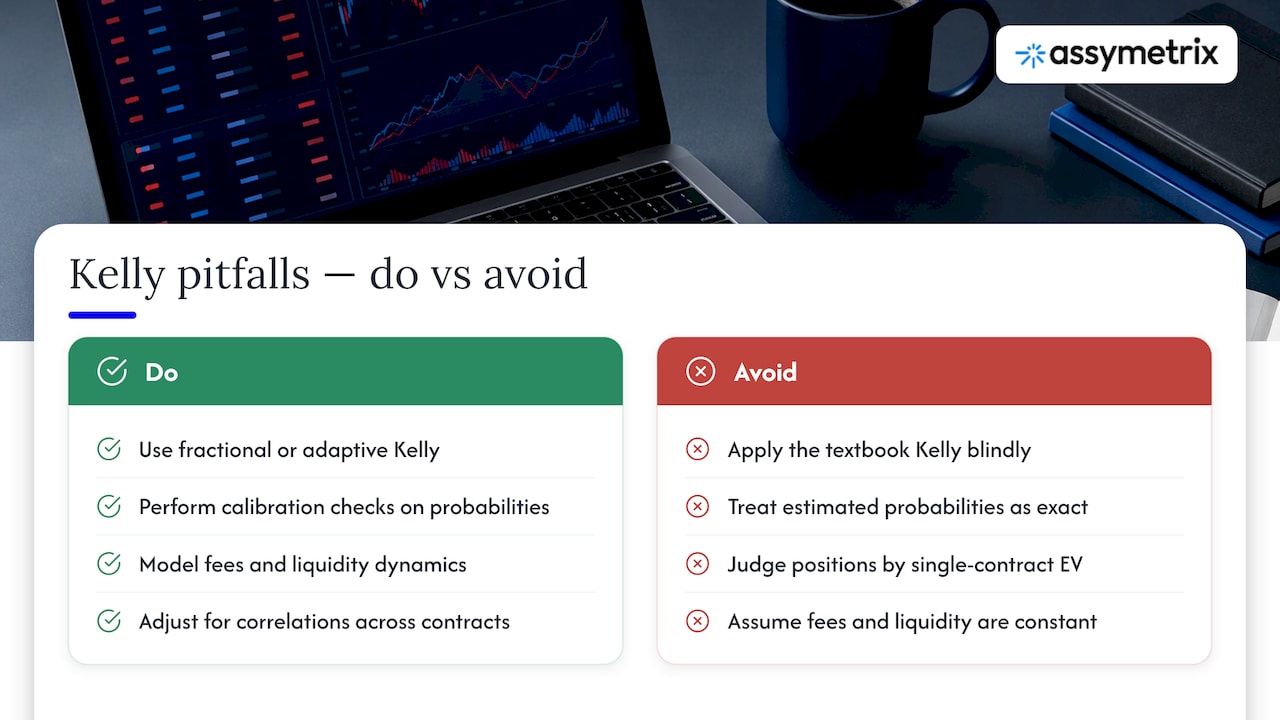
Kelly’s guarantees rest on knowing the true probability q, and no trader ever actually knows it. Every input is an estimate, and the formula has no mechanism for expressing doubt about its own inputs, which is why fractional and adaptive variants exist in the first place rather than as an optional refinement.
A second pitfall is horizon mismatch: Kelly’s optimality is a long-run, many-bet-sequence result, but most traders care about performance over a finite stretch of months or a single election cycle, where the variance around the theoretical growth path can produce outcomes far from the expected trajectory. A third is that fee structures and liquidity constraints are not static, so a sizing rule calibrated against last quarter’s fee schedule can silently overstate edge today.
A subtler failure mode involves exclusive contract families, where the Kelly-optimal allocation can in rare cases call for a hedge-like position with a negative naive expected value, a result that looks like a bug but follows from the shadow-price structure of the joint optimization. Traders who only check single-contract expected value will discard these positions and unknowingly reduce portfolio-level growth.
None of this makes Kelly the wrong framework. It makes blind application of the textbook formula, without calibration checks, fee modeling, and correlation adjustments, the actual source of most reported Kelly failures in applied betting literature.
Author’s perspective on applying Kelly in practice
We start every new model at quarter-Kelly and only scale toward half-Kelly once calibration metrics hold steady across several distinct market regimes, not one winning stretch. Backtest against real cross-venue snapshots before trusting any fraction above that.
— Dean
FAQ
What are the top prediction markets for quant trading?
Polymarket, Kalshi, and Limitless are among the most actively traded prediction market venues for quantitative strategies, each with distinct fee structures and liquidity profiles. Cross-venue coverage matters for Kelly sizing because the same event can price differently across platforms, creating both calibration checks and arbitrage signals.
What is the downside of the Kelly criterion?
Full Kelly can produce severe drawdowns, sometimes exceeding half of bankroll, even when the underlying probability model is correct on average. The formula also has no built-in way to express uncertainty about its own probability input, which is why fractional and adaptive variants are standard in applied settings.
Can you actually make money on prediction markets?
Profitability depends on having a probability model with a real, fee-adjusted edge over market prices, which is harder to sustain than it sounds once fees and favorite-longshot bias are accounted for. Traders who track calibration metrics and size with fractional Kelly tend to survive the inevitable losing streaks that a positive-edge strategy still produces.
Does Warren Buffett use the Kelly criterion?
Buffett has not published a formal endorsement of the Kelly criterion as a sizing rule for his own investment decisions. Some investors and commentators have drawn parallels between concentrated, high-conviction position sizing and Kelly-style logic, but this is an inference rather than a documented practice.
How do fees affect Kelly sizing on prediction markets?
Platform fees shrink the effective edge used in the Kelly formula and create a no-trade band around fair value where small edges are not worth betting at all. Adjusting the market price to an effective price that includes expected commission, as described in prediction market fee research, is a necessary step before applying any Kelly fraction.
Sources
Optimal sports betting strategies in practice: an experimental review
How do prediction market fees affect prices and participants? (MPRA)
Get cross-venue data built for Kelly sizing
Every formula in this guide depends on one input traders underestimate: the quality and completeness of the price and probability data feeding q and p. Our Data API solves that specific bottleneck by aggregating real-time and historical trading activity across major prediction market venues into a single normalized schema, providing extensive historical data so you are not reconciling multiple venue schemas before you can even start calibrating a model.
Beyond raw price history, we surface Smart Money wallet tracking, Trader Skill Scores, and cross-venue divergence signals that feed directly into the calibration and correlation checks this guide recommends before scaling a Kelly fraction. Our cross-venue data API gives developers, quant researchers, and algorithmic bot builders a single integration point instead of three separate venue connections to maintain. If your next step is backtesting a fractional Kelly model against real historical snapshots, start by pulling canonical cross-venue data rather than building your own normalization layer from scratch.
For traders who want an external perspective on conservative fraction selection and simulator-based testing before committing real capital, practical guidance on Kelly fractions and simulation testing covers position-sizing discipline from a trading-education angle that complements the math here.
Scale Kelly Betting for Prediction Market Quants: Large N & Data API
Adaptive fractional Kelly, not full Kelly, is the right default for prediction market sizing: shrink your bet fraction to reflect calibration uncertainty and model fees before you ever post size. Three forces drive this: estimation error in your probability model, platform fees and liquidity limits, and the scaling burden of running many simultaneous positions. The math and a working implementation checklist follow below.
TL;DR:
Fractional Kelly sizing, such as quarter or half Kelly, reduces drawdowns and accounts for probability estimation errors, fees, and liquidity limits.
Adaptive Kelly strategies incorporate confidence levels, shrinking bets when model calibration is unstable or data is sparse, to avoid overbetting.
Including platform fees in the effective price and considering favorite-longshot biases minimizes overestimation of edge and false signals.
Jointly optimizing Kelly across many correlated positions requires correlation discounts or groupings to prevent overexposure and underestimated risk.
Reliable backtesting and real-time calibration monitoring are crucial to prevent overbetting due to outdated fee assumptions, biased models, or correlation misjudgments.
Assymetrixassymetrix.comBuild Kelly Strategies On Unified DataAccess cross venue prediction market data, Smart Money signals, and historical coverage through one integration for research and trading tools.Explore Assymetrix data
Table of Contents
Mathematical foundations of Kelly for binary contracts
Kelly as information-theoretic and Bayesian model evaluation
Fractional and adaptive Kelly variants for estimation risk
Multivariate Kelly and scaling to many simultaneous bets
How fees and favorite-longshot bias change sizing
Implementation checklist for data, backtests, and production sizing
Case studies: Kelly sizing in live prediction markets
Extending Kelly to correlated and dependent outcomes
Limitations and pitfalls of Kelly in prediction markets
Author’s perspective on applying Kelly in practice
Sources
Get cross-venue data built for Kelly sizing
Mathematical foundations of Kelly for binary contracts
A prediction market contract pays $1 if an event resolves “yes” and $0 otherwise, trading at price p. If your model assigns true probability q to the event, the Kelly-optimal fraction of bankroll to stake is:
f* = (q - p) / (1 - p)
when q > p (buying yes), and the mirrored form for selling. Here p is the market-implied probability, q is your subjective estimate, and f* is the share of current bankroll committed to the position. This maximizes expected log-wealth, E[log(1 + f*X)], rather than expected wealth itself, which is the detail that separates Kelly from naive expected-value maximization.
Kelly sizing is asymptotically optimal: over a long enough sequence of independent bets, no other fixed-fraction rule compounds bankroll faster. That guarantee is a limit result, though, and it says nothing about what happens over 50 or 200 bets, where variance around the growth-optimal path can be severe.
A few corollaries matter more in practice than the formula itself:
Full Kelly maximizes long-run growth rate but comes with drawdowns that can exceed 50% of bankroll even when every probability estimate is correct.
Fractional Kelly trades some growth rate for a large reduction in variance, which is usually the better trade when q is itself uncertain.
The formula is only as good as q: a biased or overconfident probability model turns the Kelly rule into a precise instruction to overbet.
Kelly as information-theoretic and Bayesian model evaluation
Kelly’s objective decomposes cleanly into three pieces: a money term reflecting the realized payoff, an entropy term tied to the market’s own uncertainty, and a Kullback-Leibler divergence term that measures the gap between your model’s distribution and the true one. The information-theoretic framing of Kelly shows that reducing this KL divergence is the direct lever that increases long-run growth, independent of any particular bet’s outcome.
This gives Kelly a second identity: it behaves like an online Bayesian evaluation of competing models. Wealth compounds in proportion to how well a model’s implied probabilities track the posterior plausibility of outcomes, so a trader running multiple models in parallel effectively lets Kelly-weighted capital allocation reveal which model is best calibrated over time.
Two practical points follow:
Track a rolling KL-like calibration metric (such as log-loss against realized outcomes) rather than win rate alone.
Only increase your bet fraction toward full Kelly when that calibration metric has been stable across multiple market regimes, not just a single winning streak.
Fractional and adaptive Kelly variants for estimation risk
An experimental review of applied Kelly strategies finds that full Kelly is routinely too aggressive once estimation error in q is accounted for, and that fractional or adaptive variants perform better out of sample across betting domains including sports markets.
Adaptive schemes go further by letting c move with your confidence in q:
Apply posterior shrinkage, pulling q toward the market price p when your model’s sample size is small.
Temper older observations with a discount factor so stale data carries less weight in the current probability estimate.
Scale c down directly as a function of the variance of your q estimate, so wider confidence intervals mechanically produce smaller bets.
Pro Tip: Before raising your Kelly fraction, run a bootstrap on your q estimates and confirm the resulting confidence interval does not cross the market price p; if it does, the edge is not statistically distinguishable from zero.
Validation before deployment should include calibration plots across probability buckets, bootstrap confidence intervals for q, and an explicit cap on maximum drawdown that forces a fraction step-down when breached.
Multivariate Kelly and scaling to many simultaneous bets
Running Kelly across dozens or hundreds of concurrent prediction market positions is a different problem than sizing one contract. The multivariate Kelly objective requires jointly optimizing a vector of bet fractions to maximize expected log-wealth across all positions at once, and a naive solver that enumerates outcome combinations scales exponentially with the number of simultaneous contracts, N.
Two methods make this tractable. The efficient multivariate Kelly optimization approach introduces an integral-transform method that reduces per-evaluation cost to roughly linear in N when bets are close to independent, alongside a decomposition technique that builds subproblem lower and upper bounds with greedy constructions for cases where independence does not hold cleanly.
In practice:
Use the subproblem lower-bound construction first; it is fast and gives a conservative allocation you can deploy immediately.
Check shortfall-ratio diagnostics between the lower and upper bounds to see how much growth you are leaving on the table.
When N grows into the hundreds, fall back to a greedy heuristic allocation rather than waiting on an exact solver that will not finish before markets move.
How fees and favorite-longshot bias change sizing
Platform fees do not just shave expected value, they create a no-trade band around fair value where no bet is worth placing at all. The MPRA analysis of prediction market fees models this directly and shows post-fee loss rates vary with contract probability, with fee structures similar to Kalshi’s effectively acting like a charge of around 7% on winnings.
To fold this into Kelly sizing:
Convert the raw market price into an effective price, p_effective, that includes expected commission on winnings and the bid-ask spread you expect to pay.
Compute edge_after_fees = q - p_effective rather than q - p, and run that adjusted edge through the fractional Kelly formula.
Drop any position where edge_after_fees falls below a minimum threshold set by your expected slippage and fee drag, since fee-eroded edges below that line are not worth the capital at risk.
Favorite-longshot bias compounds this: longshot contracts tend to be systematically overpriced relative to true probability, so the same raw edge is worth less after fees on a longshot than on a near-coin-flip contract.
Implementation checklist for data, backtests, and production sizing
A Kelly pipeline is only as reliable as the data feeding it. The minimum input set is canonical contract identifiers that resolve consistently across venues, top-of-book quotes, time-series snapshots for historical calibration, and wallet-level trading signals that flag informed flow. Cross-venue normalization matters because the same event can trade under different schemas on Polymarket, Kalshi, and Limitless, and an unnormalized pipeline will silently double-count or miss arbitrage-relevant price divergence.
The backtest recipe that holds up in practice: walk-forward splits rather than a single train-test cut, bootstrap confidence intervals around your q estimates, explicit fee and slippage modeling for every simulated fill, and stress tests that replay historical drawdown periods rather than just average-case paths.
In production, the loop runs model to edge_after_fees to a fractional Kelly sizing module to execution filters that check liquidity depth before committing size. A backtesting workflow built on large-scale price snapshot data is a reasonable template for walk-forward testing at this stage.
Pull canonical IDs and order-book depth from a cross-venue data feed before building any calibration model.
Monitor calibration drift continuously and step the Kelly fraction down automatically when the rolling log-loss metric worsens.
Pro Tip: Treat your fraction c as a live parameter tied to a calibration dashboard, not a constant you set once and forget.
Case studies: Kelly sizing in live prediction markets
Applied reviews of Kelly in betting markets consistently point to the same pattern: traders who ran full Kelly on sports and prediction contracts experienced sharper peak-to-trough drawdowns than those running half-Kelly or quarter-Kelly, even when both groups had similarly profitable models over the full sample. The experimental review of optimal betting strategies documents this directly, recommending fractional and risk-adjusted Kelly variants as the practical standard rather than the textbook formula.
A representative illustrative scenario: say a trader’s model assigns q = 0.60 to a binary contract trading at p = 0.52, before fees. Full Kelly would call for f* = (0.60 - 0.52) / (1 - 0.52), or roughly 0.167 of bankroll, on that single position.
The broader lesson from applied reviews is not that Kelly fails in prediction markets. It is that the formula’s output is a ceiling, and treating it as a fixed instruction rather than an upper bound is the most common operational mistake traders make when moving from backtest to live capital.
Extending Kelly to correlated and dependent outcomes
Prediction markets rarely offer truly independent bets. Multiple contracts tied to the same election, the same economic release, or the same sports season share underlying risk factors, and treating them as independent when sizing positions understates portfolio-level risk.
The multivariate Kelly framework handles this by optimizing a joint fraction vector rather than sizing each contract in isolation, which is precisely why the integral-transform and decomposition methods matter beyond pure computational convenience. When bets are correlated, the decomposition approach’s subproblem bounds reveal how much the optimal joint allocation differs from the sum of individually-optimal fractions, often substantially lower, since correlated losses compound rather than diversify away.
A practical approximation when full joint optimization is not feasible: group contracts by their shared risk factor (the same election, the same macro release) and apply a correlation discount to the aggregate fraction allocated to each group, shrinking total exposure to any single correlated cluster below what the sum of individual Kelly fractions would suggest.
Limitations and pitfalls of Kelly in prediction markets
Kelly’s guarantees rest on knowing the true probability q, and no trader ever actually knows it. Every input is an estimate, and the formula has no mechanism for expressing doubt about its own inputs, which is why fractional and adaptive variants exist in the first place rather than as an optional refinement.
A second pitfall is horizon mismatch: Kelly’s optimality is a long-run, many-bet-sequence result, but most traders care about performance over a finite stretch of months or a single election cycle, where the variance around the theoretical growth path can produce outcomes far from the expected trajectory. A third is that fee structures and liquidity constraints are not static, so a sizing rule calibrated against last quarter’s fee schedule can silently overstate edge today.
A subtler failure mode involves exclusive contract families, where the Kelly-optimal allocation can in rare cases call for a hedge-like position with a negative naive expected value, a result that looks like a bug but follows from the shadow-price structure of the joint optimization. Traders who only check single-contract expected value will discard these positions and unknowingly reduce portfolio-level growth.
None of this makes Kelly the wrong framework. It makes blind application of the textbook formula, without calibration checks, fee modeling, and correlation adjustments, the actual source of most reported Kelly failures in applied betting literature.
Author’s perspective on applying Kelly in practice
We start every new model at quarter-Kelly and only scale toward half-Kelly once calibration metrics hold steady across several distinct market regimes, not one winning stretch. Backtest against real cross-venue snapshots before trusting any fraction above that.
— Dean
FAQ
What are the top prediction markets for quant trading?
Polymarket, Kalshi, and Limitless are among the most actively traded prediction market venues for quantitative strategies, each with distinct fee structures and liquidity profiles. Cross-venue coverage matters for Kelly sizing because the same event can price differently across platforms, creating both calibration checks and arbitrage signals.
What is the downside of the Kelly criterion?
Full Kelly can produce severe drawdowns, sometimes exceeding half of bankroll, even when the underlying probability model is correct on average. The formula also has no built-in way to express uncertainty about its own probability input, which is why fractional and adaptive variants are standard in applied settings.
Can you actually make money on prediction markets?
Profitability depends on having a probability model with a real, fee-adjusted edge over market prices, which is harder to sustain than it sounds once fees and favorite-longshot bias are accounted for. Traders who track calibration metrics and size with fractional Kelly tend to survive the inevitable losing streaks that a positive-edge strategy still produces.
Does Warren Buffett use the Kelly criterion?
Buffett has not published a formal endorsement of the Kelly criterion as a sizing rule for his own investment decisions. Some investors and commentators have drawn parallels between concentrated, high-conviction position sizing and Kelly-style logic, but this is an inference rather than a documented practice.
How do fees affect Kelly sizing on prediction markets?
Platform fees shrink the effective edge used in the Kelly formula and create a no-trade band around fair value where small edges are not worth betting at all. Adjusting the market price to an effective price that includes expected commission, as described in prediction market fee research, is a necessary step before applying any Kelly fraction.
Sources
Optimal sports betting strategies in practice: an experimental review
How do prediction market fees affect prices and participants? (MPRA)
Get cross-venue data built for Kelly sizing
Every formula in this guide depends on one input traders underestimate: the quality and completeness of the price and probability data feeding q and p. Our Data API solves that specific bottleneck by aggregating real-time and historical trading activity across major prediction market venues into a single normalized schema, providing extensive historical data so you are not reconciling multiple venue schemas before you can even start calibrating a model.
Beyond raw price history, we surface Smart Money wallet tracking, Trader Skill Scores, and cross-venue divergence signals that feed directly into the calibration and correlation checks this guide recommends before scaling a Kelly fraction. Our cross-venue data API gives developers, quant researchers, and algorithmic bot builders a single integration point instead of three separate venue connections to maintain. If your next step is backtesting a fractional Kelly model against real historical snapshots, start by pulling canonical cross-venue data rather than building your own normalization layer from scratch.
For traders who want an external perspective on conservative fraction selection and simulator-based testing before committing real capital, practical guidance on Kelly fractions and simulation testing covers position-sizing discipline from a trading-education angle that complements the math here.
Other Blog


