Bayesian Updating: 3 Experiments for Quants in Prediction Markets
Bayesian Updating: 3 Experiments for Quants in Prediction Markets
Bayesian Updating: 3 Experiments for Quants in Prediction Markets
How quants and devs deploy Bayesian updating in prediction markets: log odds math, calibrated likelihoods, RN JD volatility modeling, and production...

Bayesian Updating: 3 Experiments for Quants in Prediction Markets
Use the market price as your prior, convert it to log-odds, apply a likelihood ratio for each new piece of evidence, then trade when your posterior exceeds the market price. That is the entire operational engine of Bayesian updating in prediction markets. The math is a century old; what makes it work in 2026 is disciplined implementation: numerically stable log-odds arithmetic, honest likelihood calibration, and enough engineering rigor to filter microstructure noise, model state-dependent volatility, and avoid stacking correlated bets across related contracts.
TL;DR:
Proper calibration of prior strength based on liquidity and time-to-resolution is essential to avoid overconfidence in thin or long-dated markets.
Converting prices to log-odds and applying likelihood ratios additively reduces numerical errors and improves Bayesian updating near probabilities of 0 or 1.
Assigning likelihood ratios to evidence sources must be recalibrated regularly and validated against realized outcomes to prevent miscalibration and false edges.
Cross-venue price comparisons help identify unreliable priors caused by low liquidity or strategic trader behavior, improving evidence trustworthiness.
Market-making strategies should adapt spreads and inventory limits based on explicit belief uncertainty, trade flow consistency, and impending resolution deadlines.
Table of Contents
Bayesian Updating Prediction Markets: The Odds and Log-Odds Math
Building the Trading Loop: From Prior to Position Size
Bayesian Market-Making: Adaptive Spreads and Inventory Control
Prediction Markets as Bayesian Inverse Problems
Belief Volatility, Jumps, and the RN-JD Calibration Pipeline
Data Engineering for Bayesian Pipelines
Bayesian Updating for Prediction Markets: Next Steps Checklist
Where Bayesian Updating Breaks Down in Practice
Bayesian Updating Versus Alternative Belief-Revision Methods
Liquidity, Trader Behavior, and When Updates Are Trustworthy
Editorial Take: What the Research Actually Supports
Sources
Bayesian Updating Prediction Markets: The Odds and Log-Odds Math
Every Bayesian update in a binary prediction market reduces to one identity. Given a prior probability ( p_0 ) and new evidence HE, the posterior odds equal the prior odds times the likelihood ratio:
$$\frac{p_1}{1-p_1} = \frac{p_0}{1-p_0} \times \frac{P(E \mid \text{Yes})}{P(E \mid \text{No})}$$
The market price, treated as a probability, is the prior. The likelihood ratio (LR) is whatever weight you assign to the new information: a poll crossing a threshold, a data release, a wallet-tagged trade cluster. If a contract trades at 30% and a confirming signal carries an LR of 3, posterior odds move from $0.3/0.7 = 0.43$ to $0.43 \times 3 = 1.29$, which converts back to a posterior probability of roughly 56%. That 26-point gap between posterior and market price is your raw edge, before transaction costs and slippage.
Why log-odds, not raw probability
Odds-form Bayes works, but it breaks down numerically near the boundaries. Probabilities close to 0 or 1 compress into a tiny numeric range, and repeated multiplication of likelihood ratios in that range produces rounding errors that quietly distort your posterior. The fix is the logit transform: $x = \ln\left(\frac{p}{1-p}\right)$.
In log-odds space, Bayesian updating becomes additive rather than multiplicative:
$$x_1 = x_0 + \ln(\text{LR})$$
Every update is a simple sum. This is not a cosmetic convenience. The Bayesian inverse-problem framing of prediction markets shows that additive log-odds updates, paired with a state-dependent variance term, materially reduce overconfidence as contracts approach resolution, exactly the regime where probabilities pile up near 0 or 1 and naive arithmetic is least trustworthy.
Beta-Binomial conjugacy and encoding prior strength
When your evidence arrives as a stream of binary outcomes (correct call/incorrect call, confirmed/denied), the Beta-Binomial conjugate pair gives you a closed-form update. Model the market price as a Beta($\alpha_0$, $\beta_0$) prior, where $\alpha_0 = p_0 \cdot n_0$ and $\beta_0 = (1-p_0) \cdot n_0$. The parameter $n_0$ is your effective sample size, essentially how much weight you assign to the market’s current price versus your incoming evidence. After observing OK successes in and trials, the posterior is simply Beta($\alpha_0 + k$, $\beta_0 + n - k$).
Choosing $n_0$ is a judgment call grounded in liquidity and time to resolution. A thinly traded, long-dated contract deserves a low $n_0$, since the market price reflects fewer informed participants. A deep, actively traded market close to resolution deserves a high $n_0$, because the price already encodes a dense information set that new evidence rarely overturns wholesale.
When conjugacy fails
Not every evidence source arrives as clean binary counts. Continuous signals, like a probability estimate from a forecasting model or a sentiment score derived from news text, require converting the signal into an equivalent likelihood ratio rather than a conjugate update. The practical approach is to bucket the continuous signal into calibrated bands (strong confirming, weak confirming, neutral, weak disconfirming, strong disconfirming) and assign each band a fixed LR based on historical calibration. When no clean conjugate form exists, numerical approximation via grid evaluation of the posterior over a fine probability lattice is usually cheaper to implement correctly than deriving an analytic non-conjugate update, and it is far less error-prone for a production system running thousands of markets simultaneously.
Building the Trading Loop: From Prior to Position Size
The math only pays off when it is wired into a repeatable loop: observe price, form prior, ingest evidence, compute likelihood, update, size, log. Here is that loop in the order a trading system actually executes it.
Pull the current mid price for the contract and convert it to log-odds using $x_0 = \ln(p/(1-p))$. This is your prior.
Set prior strength using the effective sample-size heuristic: assign higher $n_0$ to liquid, near-resolution markets, and lower $n_0$ to thin or long-dated ones, since a thin market’s price reflects fewer informed participants and deserves less trust.
Classify the incoming evidence (poll, official data release, expert report, or order-flow signal) and assign a likelihood ratio. Practitioner heuristics commonly use LR bands ranging from moderate to strong for confirming polls or data releases, and correspondingly lower bands for weaker confirming signals and their disconfirming counterparts.
Apply the update additively in log-odds space: $x_1 = x_0 + \ln(\text{LR})$, then convert back to probability for interpretation.
Check for sequential and correlated evidence. If a second signal is not independent of the first, discount its likelihood ratio rather than applying it at full weight, or you will double-count the same underlying information across two “separate” updates.
Compute your edge: posterior probability minus market price. If posterior exceeds price, you have a directional edge on Yes; if it falls below, the edge favors No.
Size the position with fractional Kelly. Full Kelly sizing (of^* = \text{edge}/\text{odds}$) is too aggressive given model uncertainty, so most quant desks run at one-quarter to one-half Kelly. A 10-point edge on a contract priced at 40 cents, sized at half-Kelly, might translate to roughly 8% to 12% of bankroll rather than the 20%+ full Kelly would suggest.
Log the trade: prior, evidence description, assigned LR, posterior, market price at execution, and position size. This update log becomes your calibration dataset.
Correlation discounting deserves special attention because it is where most homegrown Bayesian systems quietly leak edge. If you are trading a Fed rate decision market and a related inflation-expectations market off the same jobs report, updating both markets at full LR from the same data release effectively double-counts one piece of information as two. The inverse-problem literature on prediction markets treats this with volume-gated mixtures that separate genuine new information from correlated repricing across related contracts. In practice, a simpler discount factor, applied by hand, based on the historical correlation between the two markets’ price series, gets most of the benefit without the modeling overhead.
Pro Tip: Keep a running column in your update log for “LR realized vs. LR assigned.” Every time a market resolves, back-calculate what likelihood ratio your evidence should have carried given the outcome, and compare it to what you assigned in real time. This single column is the fastest way to discover that your “strong confirming poll” heuristic is actually only worth an LR of 2, not the 5 you have been using.
The telemetry matters as much as the math. A system that updates beliefs correctly but never records why it updated cannot improve its likelihood heuristics, and likelihood miscalibration, not the Bayesian framework itself, is the most common source of underperformance in practitioner-built updaters.
Bayesian Market-Making: Adaptive Spreads and Inventory Control
Bayesian updating does not only inform directional trades. It also defines how a market maker should quote. The classic logarithmic market scoring rule (LMSR) sets prices from a fixed cost function regardless of the maker’s actual belief uncertainty or inventory position, which leaves it structurally exposed when informed order flow arrives in bursts.
Adaptive Bayesian Market Maker (BMM) designs fix this by treating the maker’s belief as a probability distribution with explicit variance, not a point estimate. As trades arrive, the maker updates both its mean belief and its confidence in that belief, widening spreads when trade flow looks inconsistent (a sign of adverse selection) and narrowing them when flow looks consistent with the maker’s own posterior. Experimental evaluation of BMM designs shows faster convergence to true value during belief jumps while controlling expected loss compared to static LMS-style schemes.
Stochastic-control formulations push this further by making optimal quotes a function of four state variables simultaneously: current inventory, the maker’s latent belief, time remaining to resolution, and risk aversion. The optimal market-making framework for prediction markets derives quotes via a Hamilton-Jacobi-Bellman equation and demonstrates materially better downside protection than myopic quoting benchmarks that ignore inventory and time-to-resolution jointly.
For anyone building a maker bot rather than just consuming quotes, this has direct engineering consequences:
Quote width should scale with a rolling trade-consistency index, not a fixed basis-point spread, since flow that contradicts your posterior signals adverse selection risk.
Cancel and requite logic needs a shorter refresh window near resolution, when belief volatility spikes and stale quotes get picked off.
Inventory limits should tighten as time-to-resolution shrinks, mirroring how options market makers de-risk gamma exposure into expiry.
Risk controls should track realized variance against the maker’s own posited belief-variance, flagging regimes where realized moves are outrunning the model.
None of this requires abandoning a simpler cost-function approach entirely. It requires recognizing that a maker quoting on log-odds beliefs with explicit uncertainty tracking will out-survive a static-spread maker whenever informed flow concentrates around news events, which in prediction markets is most of the time.
Prediction Markets as Bayesian Inverse Problems
Directional trading treats the market price as your prior. Research reframes the entire market as the object of inference: given a full price-volume history, what latent belief distribution and trader-type mixture generated it?
The Bayesian inverse-problem formulation of prediction markets models observed log-odds price movements as noisy signals of a latent belief process, with a volume-gated mixture separating informed traders from noise traders. This mechanism-agnostic setup does not assume you know the exact trading rule generating prices. Instead, it treats the price-volume series as data and asks what latent parameters make that data most probable, the same inverse-problem logic used in geophysical tomography or medical imaging reconstruction.
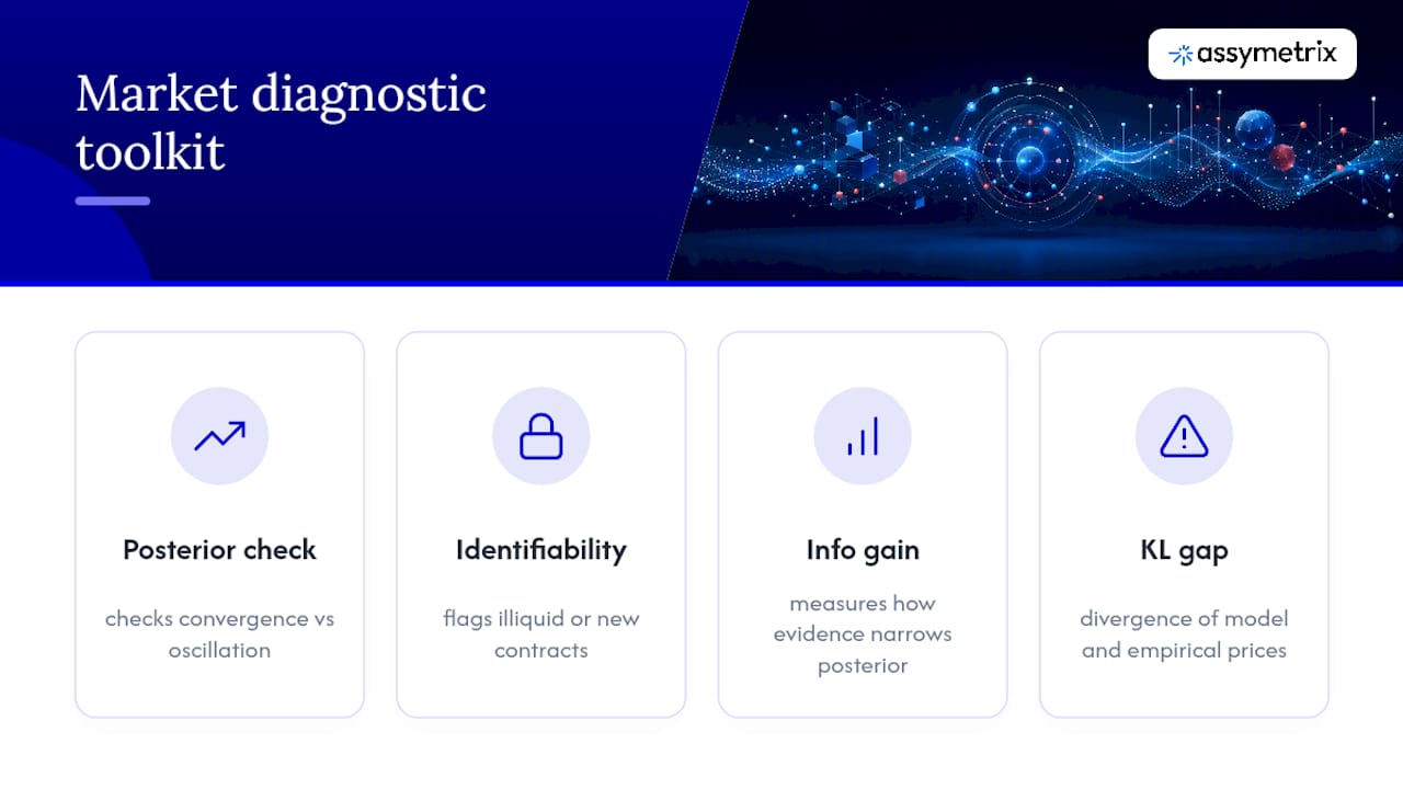
One diagnostic from this framework stands out for practical use: the KL-projection gap, which measures the divergence between your fitted model’s implied price distribution and the market’s actual empirical distribution. A small, stable KL gap over a rolling window indicates your likelihood model is well-specified for that market; a gap that widens sharply signals either a regime change or a market where your model’s assumptions (independence, mixture weights) have broken down.
Three diagnostics translate this framework into daily practice:
Posterior concentration checks whether repeated updates are converging to a stable belief or oscillating, a sign of either genuine uncertainty or a misspecified likelihood. Identifiability thresholds flag markets where price and volume jointly fail to pin down the latent parameters tightly enough for the posterior to be trustworthy, common in illiquid or newly listed contracts. Information-gain metrics quantify how much each new evidence source is actually narrowing the posterior, letting you retire likelihood heuristics that consistently contribute near-zero information gain despite feeling intuitively important.
Markets that fail these diagnostics, thin volume, erratic KL gaps, low identifiability, are exactly the markets where a naive Bayesian updater is most likely to generate false-positive edges. Treat diagnostic failure as a hard filter before sizing any position, not a footnote.
Belief Volatility, Jumps, and the RN-JD Calibration Pipeline
Log-odds prices do not move like a smooth diffusion. They jump on scheduled releases, drift between them, and accelerate as resolution approaches. Capturing that behavior requires a structural volatility model, not a flat variance assumption.
The approach maps the price up to $x = \text{logit}(p)$ and models ex as a jump-diffusion process under a risk-neutral drift, an architecture the unified kernel framework for prediction markets calls an RN-JD kernel. The diffusion component captures gradual belief drift from ordinary order flow; the jump component captures discrete belief revisions from data releases, news, or resolution-adjacent information cascades.
Calibrating this kernel means estimating a belief-volatility surface, analogous to an implied-volatility surface in options markets, and separating the diffusion and jump components in the observed price series. The standard pipeline filters microstructure noise first, then applies an EM algorithm to assign each price move a probability of being diffusion versus jump, iterating until the component parameters stabilize. Co-jump detection across related markets (two contracts that both jump on the same news event) is a useful cross-check: genuine information jumps tend to co-occur across correlated contracts, while noise-driven jumps in one market typically do not propagate.
This matters for updating because it directly explains state-dependent volatility. The structural decomposition of prediction-market volatility separates variance into a deadline-resolution channel, volatility that rises mechanically as a contract nears its resolution date regardless of news flow, and an order-flow channel driven by informed trading intensity. A Bayesian updater that ignores the deadline channel will systematically overreact to price noise in the final days before resolution, precisely when raw volatility is highest but genuine information content per price tick is often lowest. Building the RN-JD belief-volatility surface into your variance estimate corrects for this, and it gives market makers a quotable belief-risk instrument for hedging exposure the same way options desks hedge vega.
Data Engineering for Bayesian Pipelines
Running this at scale requires clean inputs before any Bayesian math executes. The minimum signal set includes mid price, bid-ask spread, individual trades, rolling volume, canonical contract IDs that map equivalent markets across venues, and wallet tags for identifying informed flow.
Preprocessing should filter microstructure noise before log-odds conversion, align ticks to a consistent time grid, and maintain rolling windows sized to the market’s typical information-arrival rate for likelihood estimation. Two API patterns cover most production needs: a WebSocket stream for low-latency updates feeding live posteriors, and bulk historical exports for calibrating prior strength and likelihood ratios against realized outcomes.
Mid, bid-ask, and trade-level data feed the log-odds conversion and noise filter.
Canonical cross-venue IDs let you join equivalent Polymarket and Kalshi contracts into one belief state instead of tracking duplicates.
Wallet-level tags for Smart Money flow give you an independent likelihood signal separate from raw price movement.
Trader Skill Scores help weight whose order flow should move your posterior versus whose should be discounted as noise.
Assymetrix’s Data API normalizes these signals across Polymarket, Kalshi, and Limitless into one schema, which removes the venue-specific parsing work that otherwise eats the first month of any Bayesian pipeline build.
Bayesian Updating for Prediction Markets: Next Steps Checklist
Operate in log-odds, not raw probability. Set prior strength from liquidity and time-to-resolution, not a fixed default. Calibrate likelihood ratios against your own update log, not borrowed heuristics. Filter microstructure noise before every update. Run identifiability and KL-gap diagnostics before sizing. Size with fractional Kelly, never full Kelly.
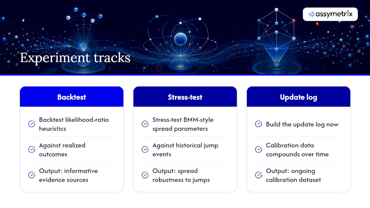
Three experiments deserve priority: backtest your likelihood-ratio heuristics against realized outcomes to find which evidence sources are actually informative, stress-test BMM-style spread parameters against historical jump events, and build the update log now, since calibration data compounds in value the longer it runs.
Where Bayesian Updating Breaks Down in Practice
The framework’s biggest failure mode is not the math. It is information aggregation error: prediction markets aggregate dispersed private signals into price, but that aggregation is only as good as the trader population’s incentives and information quality. When a market is thin or dominated by a handful of participants, the price stops functioning as a reliable prior, and treating it as one anchors your posterior to noise rather than signal.
Strategic behavior compounds the problem. Traders with an informational edge have every incentive to trade gradually rather than reveal their full belief at once, which means the price you observe understates the informed view and your likelihood-ratio updates on top of it inherit that lag. Wash trading, wallet splitting to disguise position size, and coordinated pump-style activity around low-liquidity contracts all distort the price signal your Bayesian prior depends on.
Model misspecification is the second major risk. A likelihood ratio calibrated on historical polling data may not transfer to a geopolitical event market with a fundamentally different evidence structure. The Bayesian inverse-problem framework flags this through identifiability diagnostics, but no diagnostic fully substitutes for domain-specific likelihood calibration per market category.
Finally, Bayesian updaters can be gamed by adversarial actors who understand the updater’s likelihood heuristics and manufacture evidence, a fake news cycle, a coordinated wallet cluster, specifically to trigger a predictable posterior shift. Treat any evidence source with a known, mechanical likelihood mapping as a potential attack surface, not just an information channel.
Bayesian Updating Versus Alternative Belief-Revision Methods
Bayesian updating is not the only way to revise a trading belief, and comparing it honestly against the alternatives clarifies when it earns its complexity.
Simple heuristic rules, buy when price crosses a threshold, sell on a fixed percentage move, require no probability model at all and are cheap to implement, but they cannot distinguish a genuine information event from routine noise, which is exactly the distinction a log-odds likelihood ratio is designed to make.
Frequentist statistical arbitrage, running a regression or a z-score model against historical price relationships, handles mean-reversion and pairs-style signals well but has no native mechanism for incorporating a single new qualitative signal, like a leaked report or an expert opinion, the way a likelihood ratio does.
Momentum and trend-following approaches assume the recent price path itself is the best predictor of the next move. They work well in genuinely trending regimes but systematically lag at inflection points, precisely where a Bayesian updater conditioning on new external evidence gets ahead of the price.
The comparative edge of Bayesian updating is its explicit separation of prior, evidence, and posterior, which makes every belief revision auditable and back testable against an update log. Alternative methods often blend these components implicitly, which makes it harder to diagnose why a strategy is losing edge when live likelihood calibration drifts from back tested calibration. That auditability is the practical reason quant desks default to the Bayesian frame even when a simpler heuristic would trade similarly most of the time.
Liquidity, Trader Behavior, and When Updates Are Trustworthy
A Bayesian posterior is only as reliable as the price it starts from, and price reliability is a direct function of liquidity depth and the composition of who is trading.
In deep, actively traded markets, price responds to genuine information with tight bid-ask spreads and continuous two-sided flow, which is exactly the environment where treating price as a high-confidence prior (a high $n_0$ in the Beta-Binomial framing) is justified. In thin markets, a single large order can move price several points without reflecting any new information at all, which means your prior strength assumption needs to drop sharply or your updater will mistake a liquidity shock for a belief shock.
Trader composition matters as much as depth. A market dominated by a handful of large, informed wallets will show price moves that are genuinely information-rich, worth a high likelihood ratio when they align with your own evidence. A market with heavy retail-style flow and low Trader Skill Scores across the active wallet base will show price moves that are noisier relative to fundamentals, meaning the same size price move deserves a lower likelihood weight before you fold it into a posterior.
This is why cross-venue data matters for reliability, not just coverage. The same event often trades on both Polymarket and Kalshi with different liquidity profiles and different trader populations. Comparing posteriors derived independently of each venue, rather than trusting a single venue’s price as the sole prior, surfaces divergence that either flags an arbitrage opportunity or, more usefully for calibration purposes, flags a venue where the price is currently a less trustworthy prior than the other. Cross-venue arbitrage signal work built on normalized order-book and trade data makes this comparison tractable without manually reconciling two different market schemas.
Editorial Take: What the Research Actually Supports
The academic literature on Bayesian prediction markets has outpaced what most trading desks actually run in production. Papers on inverse-problem formulations and RN-JD kernels are solving real calibration problems, yet most practitioner systems still update on raw probability differences with no log-odds transform and no explicit treatment of state-dependent variance. That gap, not a lack of theory, is where most edge gets left on the table.
The conventional advice to “just trust the market price” undersells how much prior strength should vary by liquidity and time-to-resolution. A flat prior-strength assumption across every contract in a portfolio is the single most common modeling error I see implied in practitioner write-ups. It treats a thin, month-out contract the same as a deep, hours-from-resolution one, when those two situations call for almost opposite prior weightings.
If you take one thing from this framework, prioritize the update log before the likelihood models. Calibration data compounds. Without it, every likelihood ratio you assign is a guess dressed up as math.
— Dean
FAQ
What is Bayesian updating in prediction markets?
It is the process of treating the current market price as a prior probability, converting it to log-odds, and revising that probability using likelihood ratios from new evidence, such as polls, data releases, or order-flow signals, to produce a posterior estimate.
How do you convert market price into a Bayesian prior?
Convert the price to log-odds using $x = \ln(p/(1-p))$, then set the prior’s effective strength based on liquidity and time-to-resolution, giving deep, near-resolution markets more weight than thin or long-dated ones.
What likelihood ratio should I use for a confirming poll or data release?
Practitioner heuristics commonly use moderate to strong likelihood-ratio bands for confirming evidence, though these should be recalibrated against your own update log over time.
How does Bayesian market-making differ from LMSR?
Bayesian Market Maker designs track explicit belief uncertainty and adjust spreads based on trade-consistency signals, while standard LMSR uses a fixed cost function that does not adapt to the maker’s inventory or confidence.
What is the biggest risk in applying Bayesian updating to prediction markets?
Information aggregation errors from thin liquidity and strategic trader behavior, since a manipulated or noise-driven price undermines the prior your entire posterior calculation depends on.
Does market liquidity affect how much I should trust a Bayesian update?
Yes. Deeper markets with skilled, informed trader flow justify a stronger prior, while thin markets or those dominated by low-skill flow require discounting the price signal before updating on it.
Bayesian Updating: 3 Experiments for Quants in Prediction Markets
Use the market price as your prior, convert it to log-odds, apply a likelihood ratio for each new piece of evidence, then trade when your posterior exceeds the market price. That is the entire operational engine of Bayesian updating in prediction markets. The math is a century old; what makes it work in 2026 is disciplined implementation: numerically stable log-odds arithmetic, honest likelihood calibration, and enough engineering rigor to filter microstructure noise, model state-dependent volatility, and avoid stacking correlated bets across related contracts.
TL;DR:
Proper calibration of prior strength based on liquidity and time-to-resolution is essential to avoid overconfidence in thin or long-dated markets.
Converting prices to log-odds and applying likelihood ratios additively reduces numerical errors and improves Bayesian updating near probabilities of 0 or 1.
Assigning likelihood ratios to evidence sources must be recalibrated regularly and validated against realized outcomes to prevent miscalibration and false edges.
Cross-venue price comparisons help identify unreliable priors caused by low liquidity or strategic trader behavior, improving evidence trustworthiness.
Market-making strategies should adapt spreads and inventory limits based on explicit belief uncertainty, trade flow consistency, and impending resolution deadlines.
Table of Contents
Bayesian Updating Prediction Markets: The Odds and Log-Odds Math
Building the Trading Loop: From Prior to Position Size
Bayesian Market-Making: Adaptive Spreads and Inventory Control
Prediction Markets as Bayesian Inverse Problems
Belief Volatility, Jumps, and the RN-JD Calibration Pipeline
Data Engineering for Bayesian Pipelines
Bayesian Updating for Prediction Markets: Next Steps Checklist
Where Bayesian Updating Breaks Down in Practice
Bayesian Updating Versus Alternative Belief-Revision Methods
Liquidity, Trader Behavior, and When Updates Are Trustworthy
Editorial Take: What the Research Actually Supports
Sources
Bayesian Updating Prediction Markets: The Odds and Log-Odds Math
Every Bayesian update in a binary prediction market reduces to one identity. Given a prior probability ( p_0 ) and new evidence HE, the posterior odds equal the prior odds times the likelihood ratio:
$$\frac{p_1}{1-p_1} = \frac{p_0}{1-p_0} \times \frac{P(E \mid \text{Yes})}{P(E \mid \text{No})}$$
The market price, treated as a probability, is the prior. The likelihood ratio (LR) is whatever weight you assign to the new information: a poll crossing a threshold, a data release, a wallet-tagged trade cluster. If a contract trades at 30% and a confirming signal carries an LR of 3, posterior odds move from $0.3/0.7 = 0.43$ to $0.43 \times 3 = 1.29$, which converts back to a posterior probability of roughly 56%. That 26-point gap between posterior and market price is your raw edge, before transaction costs and slippage.
Why log-odds, not raw probability
Odds-form Bayes works, but it breaks down numerically near the boundaries. Probabilities close to 0 or 1 compress into a tiny numeric range, and repeated multiplication of likelihood ratios in that range produces rounding errors that quietly distort your posterior. The fix is the logit transform: $x = \ln\left(\frac{p}{1-p}\right)$.
In log-odds space, Bayesian updating becomes additive rather than multiplicative:
$$x_1 = x_0 + \ln(\text{LR})$$
Every update is a simple sum. This is not a cosmetic convenience. The Bayesian inverse-problem framing of prediction markets shows that additive log-odds updates, paired with a state-dependent variance term, materially reduce overconfidence as contracts approach resolution, exactly the regime where probabilities pile up near 0 or 1 and naive arithmetic is least trustworthy.
Beta-Binomial conjugacy and encoding prior strength
When your evidence arrives as a stream of binary outcomes (correct call/incorrect call, confirmed/denied), the Beta-Binomial conjugate pair gives you a closed-form update. Model the market price as a Beta($\alpha_0$, $\beta_0$) prior, where $\alpha_0 = p_0 \cdot n_0$ and $\beta_0 = (1-p_0) \cdot n_0$. The parameter $n_0$ is your effective sample size, essentially how much weight you assign to the market’s current price versus your incoming evidence. After observing OK successes in and trials, the posterior is simply Beta($\alpha_0 + k$, $\beta_0 + n - k$).
Choosing $n_0$ is a judgment call grounded in liquidity and time to resolution. A thinly traded, long-dated contract deserves a low $n_0$, since the market price reflects fewer informed participants. A deep, actively traded market close to resolution deserves a high $n_0$, because the price already encodes a dense information set that new evidence rarely overturns wholesale.
When conjugacy fails
Not every evidence source arrives as clean binary counts. Continuous signals, like a probability estimate from a forecasting model or a sentiment score derived from news text, require converting the signal into an equivalent likelihood ratio rather than a conjugate update. The practical approach is to bucket the continuous signal into calibrated bands (strong confirming, weak confirming, neutral, weak disconfirming, strong disconfirming) and assign each band a fixed LR based on historical calibration. When no clean conjugate form exists, numerical approximation via grid evaluation of the posterior over a fine probability lattice is usually cheaper to implement correctly than deriving an analytic non-conjugate update, and it is far less error-prone for a production system running thousands of markets simultaneously.
Building the Trading Loop: From Prior to Position Size
The math only pays off when it is wired into a repeatable loop: observe price, form prior, ingest evidence, compute likelihood, update, size, log. Here is that loop in the order a trading system actually executes it.
Pull the current mid price for the contract and convert it to log-odds using $x_0 = \ln(p/(1-p))$. This is your prior.
Set prior strength using the effective sample-size heuristic: assign higher $n_0$ to liquid, near-resolution markets, and lower $n_0$ to thin or long-dated ones, since a thin market’s price reflects fewer informed participants and deserves less trust.
Classify the incoming evidence (poll, official data release, expert report, or order-flow signal) and assign a likelihood ratio. Practitioner heuristics commonly use LR bands ranging from moderate to strong for confirming polls or data releases, and correspondingly lower bands for weaker confirming signals and their disconfirming counterparts.
Apply the update additively in log-odds space: $x_1 = x_0 + \ln(\text{LR})$, then convert back to probability for interpretation.
Check for sequential and correlated evidence. If a second signal is not independent of the first, discount its likelihood ratio rather than applying it at full weight, or you will double-count the same underlying information across two “separate” updates.
Compute your edge: posterior probability minus market price. If posterior exceeds price, you have a directional edge on Yes; if it falls below, the edge favors No.
Size the position with fractional Kelly. Full Kelly sizing (of^* = \text{edge}/\text{odds}$) is too aggressive given model uncertainty, so most quant desks run at one-quarter to one-half Kelly. A 10-point edge on a contract priced at 40 cents, sized at half-Kelly, might translate to roughly 8% to 12% of bankroll rather than the 20%+ full Kelly would suggest.
Log the trade: prior, evidence description, assigned LR, posterior, market price at execution, and position size. This update log becomes your calibration dataset.
Correlation discounting deserves special attention because it is where most homegrown Bayesian systems quietly leak edge. If you are trading a Fed rate decision market and a related inflation-expectations market off the same jobs report, updating both markets at full LR from the same data release effectively double-counts one piece of information as two. The inverse-problem literature on prediction markets treats this with volume-gated mixtures that separate genuine new information from correlated repricing across related contracts. In practice, a simpler discount factor, applied by hand, based on the historical correlation between the two markets’ price series, gets most of the benefit without the modeling overhead.
Pro Tip: Keep a running column in your update log for “LR realized vs. LR assigned.” Every time a market resolves, back-calculate what likelihood ratio your evidence should have carried given the outcome, and compare it to what you assigned in real time. This single column is the fastest way to discover that your “strong confirming poll” heuristic is actually only worth an LR of 2, not the 5 you have been using.
The telemetry matters as much as the math. A system that updates beliefs correctly but never records why it updated cannot improve its likelihood heuristics, and likelihood miscalibration, not the Bayesian framework itself, is the most common source of underperformance in practitioner-built updaters.
Bayesian Market-Making: Adaptive Spreads and Inventory Control
Bayesian updating does not only inform directional trades. It also defines how a market maker should quote. The classic logarithmic market scoring rule (LMSR) sets prices from a fixed cost function regardless of the maker’s actual belief uncertainty or inventory position, which leaves it structurally exposed when informed order flow arrives in bursts.
Adaptive Bayesian Market Maker (BMM) designs fix this by treating the maker’s belief as a probability distribution with explicit variance, not a point estimate. As trades arrive, the maker updates both its mean belief and its confidence in that belief, widening spreads when trade flow looks inconsistent (a sign of adverse selection) and narrowing them when flow looks consistent with the maker’s own posterior. Experimental evaluation of BMM designs shows faster convergence to true value during belief jumps while controlling expected loss compared to static LMS-style schemes.
Stochastic-control formulations push this further by making optimal quotes a function of four state variables simultaneously: current inventory, the maker’s latent belief, time remaining to resolution, and risk aversion. The optimal market-making framework for prediction markets derives quotes via a Hamilton-Jacobi-Bellman equation and demonstrates materially better downside protection than myopic quoting benchmarks that ignore inventory and time-to-resolution jointly.
For anyone building a maker bot rather than just consuming quotes, this has direct engineering consequences:
Quote width should scale with a rolling trade-consistency index, not a fixed basis-point spread, since flow that contradicts your posterior signals adverse selection risk.
Cancel and requite logic needs a shorter refresh window near resolution, when belief volatility spikes and stale quotes get picked off.
Inventory limits should tighten as time-to-resolution shrinks, mirroring how options market makers de-risk gamma exposure into expiry.
Risk controls should track realized variance against the maker’s own posited belief-variance, flagging regimes where realized moves are outrunning the model.
None of this requires abandoning a simpler cost-function approach entirely. It requires recognizing that a maker quoting on log-odds beliefs with explicit uncertainty tracking will out-survive a static-spread maker whenever informed flow concentrates around news events, which in prediction markets is most of the time.
Prediction Markets as Bayesian Inverse Problems
Directional trading treats the market price as your prior. Research reframes the entire market as the object of inference: given a full price-volume history, what latent belief distribution and trader-type mixture generated it?
The Bayesian inverse-problem formulation of prediction markets models observed log-odds price movements as noisy signals of a latent belief process, with a volume-gated mixture separating informed traders from noise traders. This mechanism-agnostic setup does not assume you know the exact trading rule generating prices. Instead, it treats the price-volume series as data and asks what latent parameters make that data most probable, the same inverse-problem logic used in geophysical tomography or medical imaging reconstruction.
One diagnostic from this framework stands out for practical use: the KL-projection gap, which measures the divergence between your fitted model’s implied price distribution and the market’s actual empirical distribution. A small, stable KL gap over a rolling window indicates your likelihood model is well-specified for that market; a gap that widens sharply signals either a regime change or a market where your model’s assumptions (independence, mixture weights) have broken down.
Three diagnostics translate this framework into daily practice:
Posterior concentration checks whether repeated updates are converging to a stable belief or oscillating, a sign of either genuine uncertainty or a misspecified likelihood. Identifiability thresholds flag markets where price and volume jointly fail to pin down the latent parameters tightly enough for the posterior to be trustworthy, common in illiquid or newly listed contracts. Information-gain metrics quantify how much each new evidence source is actually narrowing the posterior, letting you retire likelihood heuristics that consistently contribute near-zero information gain despite feeling intuitively important.
Markets that fail these diagnostics, thin volume, erratic KL gaps, low identifiability, are exactly the markets where a naive Bayesian updater is most likely to generate false-positive edges. Treat diagnostic failure as a hard filter before sizing any position, not a footnote.
Belief Volatility, Jumps, and the RN-JD Calibration Pipeline
Log-odds prices do not move like a smooth diffusion. They jump on scheduled releases, drift between them, and accelerate as resolution approaches. Capturing that behavior requires a structural volatility model, not a flat variance assumption.
The approach maps the price up to $x = \text{logit}(p)$ and models ex as a jump-diffusion process under a risk-neutral drift, an architecture the unified kernel framework for prediction markets calls an RN-JD kernel. The diffusion component captures gradual belief drift from ordinary order flow; the jump component captures discrete belief revisions from data releases, news, or resolution-adjacent information cascades.
Calibrating this kernel means estimating a belief-volatility surface, analogous to an implied-volatility surface in options markets, and separating the diffusion and jump components in the observed price series. The standard pipeline filters microstructure noise first, then applies an EM algorithm to assign each price move a probability of being diffusion versus jump, iterating until the component parameters stabilize. Co-jump detection across related markets (two contracts that both jump on the same news event) is a useful cross-check: genuine information jumps tend to co-occur across correlated contracts, while noise-driven jumps in one market typically do not propagate.
This matters for updating because it directly explains state-dependent volatility. The structural decomposition of prediction-market volatility separates variance into a deadline-resolution channel, volatility that rises mechanically as a contract nears its resolution date regardless of news flow, and an order-flow channel driven by informed trading intensity. A Bayesian updater that ignores the deadline channel will systematically overreact to price noise in the final days before resolution, precisely when raw volatility is highest but genuine information content per price tick is often lowest. Building the RN-JD belief-volatility surface into your variance estimate corrects for this, and it gives market makers a quotable belief-risk instrument for hedging exposure the same way options desks hedge vega.
Data Engineering for Bayesian Pipelines
Running this at scale requires clean inputs before any Bayesian math executes. The minimum signal set includes mid price, bid-ask spread, individual trades, rolling volume, canonical contract IDs that map equivalent markets across venues, and wallet tags for identifying informed flow.
Preprocessing should filter microstructure noise before log-odds conversion, align ticks to a consistent time grid, and maintain rolling windows sized to the market’s typical information-arrival rate for likelihood estimation. Two API patterns cover most production needs: a WebSocket stream for low-latency updates feeding live posteriors, and bulk historical exports for calibrating prior strength and likelihood ratios against realized outcomes.
Mid, bid-ask, and trade-level data feed the log-odds conversion and noise filter.
Canonical cross-venue IDs let you join equivalent Polymarket and Kalshi contracts into one belief state instead of tracking duplicates.
Wallet-level tags for Smart Money flow give you an independent likelihood signal separate from raw price movement.
Trader Skill Scores help weight whose order flow should move your posterior versus whose should be discounted as noise.
Assymetrix’s Data API normalizes these signals across Polymarket, Kalshi, and Limitless into one schema, which removes the venue-specific parsing work that otherwise eats the first month of any Bayesian pipeline build.
Bayesian Updating for Prediction Markets: Next Steps Checklist
Operate in log-odds, not raw probability. Set prior strength from liquidity and time-to-resolution, not a fixed default. Calibrate likelihood ratios against your own update log, not borrowed heuristics. Filter microstructure noise before every update. Run identifiability and KL-gap diagnostics before sizing. Size with fractional Kelly, never full Kelly.
Three experiments deserve priority: backtest your likelihood-ratio heuristics against realized outcomes to find which evidence sources are actually informative, stress-test BMM-style spread parameters against historical jump events, and build the update log now, since calibration data compounds in value the longer it runs.
Where Bayesian Updating Breaks Down in Practice
The framework’s biggest failure mode is not the math. It is information aggregation error: prediction markets aggregate dispersed private signals into price, but that aggregation is only as good as the trader population’s incentives and information quality. When a market is thin or dominated by a handful of participants, the price stops functioning as a reliable prior, and treating it as one anchors your posterior to noise rather than signal.
Strategic behavior compounds the problem. Traders with an informational edge have every incentive to trade gradually rather than reveal their full belief at once, which means the price you observe understates the informed view and your likelihood-ratio updates on top of it inherit that lag. Wash trading, wallet splitting to disguise position size, and coordinated pump-style activity around low-liquidity contracts all distort the price signal your Bayesian prior depends on.
Model misspecification is the second major risk. A likelihood ratio calibrated on historical polling data may not transfer to a geopolitical event market with a fundamentally different evidence structure. The Bayesian inverse-problem framework flags this through identifiability diagnostics, but no diagnostic fully substitutes for domain-specific likelihood calibration per market category.
Finally, Bayesian updaters can be gamed by adversarial actors who understand the updater’s likelihood heuristics and manufacture evidence, a fake news cycle, a coordinated wallet cluster, specifically to trigger a predictable posterior shift. Treat any evidence source with a known, mechanical likelihood mapping as a potential attack surface, not just an information channel.
Bayesian Updating Versus Alternative Belief-Revision Methods
Bayesian updating is not the only way to revise a trading belief, and comparing it honestly against the alternatives clarifies when it earns its complexity.
Simple heuristic rules, buy when price crosses a threshold, sell on a fixed percentage move, require no probability model at all and are cheap to implement, but they cannot distinguish a genuine information event from routine noise, which is exactly the distinction a log-odds likelihood ratio is designed to make.
Frequentist statistical arbitrage, running a regression or a z-score model against historical price relationships, handles mean-reversion and pairs-style signals well but has no native mechanism for incorporating a single new qualitative signal, like a leaked report or an expert opinion, the way a likelihood ratio does.
Momentum and trend-following approaches assume the recent price path itself is the best predictor of the next move. They work well in genuinely trending regimes but systematically lag at inflection points, precisely where a Bayesian updater conditioning on new external evidence gets ahead of the price.
The comparative edge of Bayesian updating is its explicit separation of prior, evidence, and posterior, which makes every belief revision auditable and back testable against an update log. Alternative methods often blend these components implicitly, which makes it harder to diagnose why a strategy is losing edge when live likelihood calibration drifts from back tested calibration. That auditability is the practical reason quant desks default to the Bayesian frame even when a simpler heuristic would trade similarly most of the time.
Liquidity, Trader Behavior, and When Updates Are Trustworthy
A Bayesian posterior is only as reliable as the price it starts from, and price reliability is a direct function of liquidity depth and the composition of who is trading.
In deep, actively traded markets, price responds to genuine information with tight bid-ask spreads and continuous two-sided flow, which is exactly the environment where treating price as a high-confidence prior (a high $n_0$ in the Beta-Binomial framing) is justified. In thin markets, a single large order can move price several points without reflecting any new information at all, which means your prior strength assumption needs to drop sharply or your updater will mistake a liquidity shock for a belief shock.
Trader composition matters as much as depth. A market dominated by a handful of large, informed wallets will show price moves that are genuinely information-rich, worth a high likelihood ratio when they align with your own evidence. A market with heavy retail-style flow and low Trader Skill Scores across the active wallet base will show price moves that are noisier relative to fundamentals, meaning the same size price move deserves a lower likelihood weight before you fold it into a posterior.
This is why cross-venue data matters for reliability, not just coverage. The same event often trades on both Polymarket and Kalshi with different liquidity profiles and different trader populations. Comparing posteriors derived independently of each venue, rather than trusting a single venue’s price as the sole prior, surfaces divergence that either flags an arbitrage opportunity or, more usefully for calibration purposes, flags a venue where the price is currently a less trustworthy prior than the other. Cross-venue arbitrage signal work built on normalized order-book and trade data makes this comparison tractable without manually reconciling two different market schemas.
Editorial Take: What the Research Actually Supports
The academic literature on Bayesian prediction markets has outpaced what most trading desks actually run in production. Papers on inverse-problem formulations and RN-JD kernels are solving real calibration problems, yet most practitioner systems still update on raw probability differences with no log-odds transform and no explicit treatment of state-dependent variance. That gap, not a lack of theory, is where most edge gets left on the table.
The conventional advice to “just trust the market price” undersells how much prior strength should vary by liquidity and time-to-resolution. A flat prior-strength assumption across every contract in a portfolio is the single most common modeling error I see implied in practitioner write-ups. It treats a thin, month-out contract the same as a deep, hours-from-resolution one, when those two situations call for almost opposite prior weightings.
If you take one thing from this framework, prioritize the update log before the likelihood models. Calibration data compounds. Without it, every likelihood ratio you assign is a guess dressed up as math.
— Dean
FAQ
What is Bayesian updating in prediction markets?
It is the process of treating the current market price as a prior probability, converting it to log-odds, and revising that probability using likelihood ratios from new evidence, such as polls, data releases, or order-flow signals, to produce a posterior estimate.
How do you convert market price into a Bayesian prior?
Convert the price to log-odds using $x = \ln(p/(1-p))$, then set the prior’s effective strength based on liquidity and time-to-resolution, giving deep, near-resolution markets more weight than thin or long-dated ones.
What likelihood ratio should I use for a confirming poll or data release?
Practitioner heuristics commonly use moderate to strong likelihood-ratio bands for confirming evidence, though these should be recalibrated against your own update log over time.
How does Bayesian market-making differ from LMSR?
Bayesian Market Maker designs track explicit belief uncertainty and adjust spreads based on trade-consistency signals, while standard LMSR uses a fixed cost function that does not adapt to the maker’s inventory or confidence.
What is the biggest risk in applying Bayesian updating to prediction markets?
Information aggregation errors from thin liquidity and strategic trader behavior, since a manipulated or noise-driven price undermines the prior your entire posterior calculation depends on.
Does market liquidity affect how much I should trust a Bayesian update?
Yes. Deeper markets with skilled, informed trader flow justify a stronger prior, while thin markets or those dominated by low-skill flow require discounting the price signal before updating on it.
Other Blog


