Normalize Scalar Market Data for Devs & Quants, No Multiple Parsers
Normalize Scalar Market Data for Devs & Quants, No Multiple Parsers
Normalize Scalar Market Data for Devs & Quants, No Multiple Parsers
A technical primer for developers and quants on normalizing scalar prediction market feeds, building production pipelines, and avoiding clamp and revision...
Normalize Scalar Market Data for Devs & Quants, No Multiple Parsers
Scalar market data represents numeric-outcome event contracts whose payout equals a clamped linear mapping of a settled benchmark, not a single probability estimate. That distinction changes everything about how you ingest, model, and trade the data: a scalar tick is a point sample from an implied distribution, and treating it like a binary “yes” price will corrupt your backtests. The immediate implication for developers and quants is straightforward: normalize the schema, verify the resolution source, and model the outcome as a range before you write a single line of strategy code.
TL;DR:
Scalar market data reflects an expected value within a defined range using a clamped payoff formula, requiring careful normalization and handling of out-of-range settlements.
Accurate modeling demands incorporating distributional aspects, out-of-bound clamp risks, revision processes, and real-time streaming constraints.
Cross-venue normalization of contract specifications, resolution sources, and settlement details is essential to prevent misleading signals and enable reliable analysis.
Backtesting should focus on final settlement values with consistent clamp logic, treating revisions as noisy signals, and stress-testing near boundaries to avoid overestimating performance.
A unified data API that standardizes scalar and binary formats across multiple venues significantly reduces engineering overhead and improves data reliability for quantitative and AI workflows.
Assymetrixassymetrix.comNormalize Market Data OnceAssymetrix gives developers and quants unified scalar and binary prediction market data across Polymarket, Kalshi, and Limitless.Explore the data platform
Table of Contents
What Is a Scalar Prediction Market, and How Does It Differ From Binary?
Why Is Scalar Market Data Harder to Model Than Binary Data?
What Schema Fields Does a Scalar Market API Need to Return?
How Do Different Prediction Market Venues Publish Scalar Data?
How Do You Build an Integration Pipeline for Scalar Market Data?
Which Quant and AI Workflows Actually Benefit From Scalar Data?
How Does Assymetrix Normalize Scalar and Binary Prediction Market Data?
What Should You Watch for When Backtesting Scalar Strategies?
Author Perspective: What Comes Next for Scalar Markets
Get Normalized Scalar and Binary Data Through One Integration
Sources
What Is a Scalar Prediction Market, and How Does It Differ From Binary?
A scalar prediction market settles on a numeric value inside a defined range, and the contract pays out proportionally to where that value lands. A binary market resolves to one of two states, “yes” or “no,” and the payout is all or nothing. A scalar market on, say, next quarter’s inflation print doesn’t ask “will inflation exceed 3%?” It asks “where within a 0% to 6% band will inflation actually land?” and pays traders according to that position.
The math behind this is the clamp payoff formula, and every scalar contract you’ll encounter in the wild follows some version of it:
payout = clamp((actual − floor) / (cap − floor), 0, 1)
Three variables define the contract: the floor (the lowest value the market recognizes), the cap (the highest), and the settlement value (the actual observed outcome at resolution). If the settlement value lands below the floor or above the cap, the payout clamps to 0 or 1 respectively, which is why scalar contracts require special handling of out-of-range settlement that binary contracts never need to worry about.
Here’s the mechanics broken down for a working example. Say a scalar market on US nonfarm payrolls has a floor of 100,000 and a cap of 300,000. If the actual print comes in at 200,000, the payout calculates as (200,000 − 100,000) / (300,000 − 100,000) = 0.5. A print of 350,000 clamps to 1.0 even though it exceeds the cap by 50,000. A print of 50,000 clamps to 0 despite being 50,000 below the floor. Those clamps are not edge cases you can ignore. They are structural features of the contract that determine your P&L at the boundaries.
Binary markets skip all of this. A binary contract on “will the Fed cut rates in March” resolves to exactly 1 or 0 based on a single triggering event. There’s no floor, no cap, no proportional mapping. The price you observe before resolution is a probability estimate; the price a scalar market shows you before resolution is closer to an expected value of the underlying metric within the band, which is a fundamentally different statistical object to model.
Resolution mechanics matter as much as the payoff formula, and this is where a lot of naive integrations break:
Resolution source: every contract spec names an authoritative data provider (a government statistics bureau, an index provider, a specific exchange feed) and the venue’s smart contract or settlement engine reads from that source alone.
Revision rules: many economic series get revised after initial release. A contract spec should state whether it settles on the first print or a revised figure, and when.
Dispute windows: some venues hold a challenge period after initial settlement during which a result can be contested and corrected.
Precision and rounding: contract specs typically define the decimal precision used for both the floor/cap band and the final settlement comparison.
Miss any one of these four items when parsing a contract spec, and you’ll misattribute a settlement value, misclamp a payout, or trust a print that later gets revised out from under you.
Why Is Scalar Market Data Harder to Model Than Binary Data?
Binary market data gives you one number to track: an implied probability that moves between 0 and 1. Scalar market data gives you a price that represents where the market thinks the expected value sits inside a band, and extracting anything useful from that requires modeling an entire implied distribution, not a single scalar (the irony of the naming isn’t lost on anyone who works with this data daily).
The core challenge breaks into four distinct problems:
Distributional modeling, not probability estimation. A scalar price embeds information about the mean of the underlying distribution, but says nothing directly about variance, skew, or tail risk. Extracting a full belief distribution from a handful of scalar contracts at different strikes on the same underlying event requires curve-fitting techniques closer to options-market implied volatility surfaces than anything in classic binary forecasting.
Clamp and jump risk at expiry. Because payouts clamp at the boundaries, a market trading near the floor or cap behaves nonlinearly as expiry approaches. A settlement value that jumps just past the cap produces a discontinuous payoff, and if your backtest doesn’t model that discontinuity explicitly, you’ll systematically overstate or understate strategy returns near the boundaries.
Revision handling. Initial economic prints get revised, sometimes materially. A pipeline that treats the first settlement print as final will mislabel training data for any model trained on historical outcomes. The safer approach treats every initial print as a noisy, time-stamped observation, not ground truth.
Latency and streaming constraints. High-frequency agents trading scalar markets need sub-second visibility into order book changes, not just periodic snapshots, because scalar markets often have thinner liquidity than headline binary markets on the same underlying event and price discovery can be choppier.
Academic work on prediction market microstructure backs this up directly. A unified stochastic kernel approach to prediction markets proposes treating traded probabilities as martingales and building a calibration pipeline that filters microstructure noise before you can extract belief-volatility or jump-intensity surfaces. Skip that filtering step, and your “distribution” is mostly noise dressed up as signal.
Pro Tip: Never train a model directly on raw scalar ticks. Run them through a denoising or smoothing pass first, and keep both the raw and the smoothed series in storage. You will eventually need to explain a divergence between the two, and reconstructing the raw feed after the fact is far harder than storing it up front.
The revision problem deserves one more sentence of emphasis: treat every initial settlement print as a noisy, time-stamped observation rather than a final value, and compute both a point estimate and a smoothed distribution per market window for anything downstream that depends on it, a pattern borne out in recent kernel-based modeling work on prediction markets.
What Schema Fields Does a Scalar Market API Need to Return?
A production-grade scalar data feed needs a canonical schema that survives contact with three or more venues, each with its own idiosyncratic contract naming and settlement logic. The fields below represent the minimum viable schema for any pipeline that wants to run models across scalar markets without venue-specific branching logic scattered through the codebase.
event_id / market_id: stable identifiers that persist across venue-side renames or contract relistings.
floor / cap: the numeric bounds of the contract, normalized to a consistent unit (see below).
resolution_value: the final settled numeric outcome, populated only after settlement.
resolution_time: the timestamp of final settlement, distinct from the market’s close time.
implied_mean / implied_variance: derived fields computed from the current order book, not raw venue output.
raw_tick: the unmodified price as reported by the venue, preserved for audit and reconciliation.
provenance fields: resolution source URL, data provider name, and a confidence flag.
Normalization is where most of the real engineering work happens. Unit and scale conversion matters because one venue might quote a market in raw index points while another quotes the same underlying series as a percentage change. Band rebasing matters because two venues covering the same economic release sometimes choose different floor/cap ranges for what is nominally the same event, and comparing them without rebasing to a common scale produces meaningless deltas. Timestamp canonicalization matters because venues report in different time zones and precision levels, and clamp enforcement matters because you need to apply the payout formula consistently even when a venue’s own UI doesn’t show you the clamped value directly.
Quality flags close the loop on auditability. A schema should expose is_revised (whether the resolution value has changed since first reported), resolution_confidence (a categorical or numeric flag reflecting how authoritative the current settlement value is), and a provenance_url pointing to the source document or feed the settlement was drawn from. Exposing those three flags in streaming payloads lets live trading agents alter behavior the moment a market’s resolution confidence drops, rather than discovering the problem after a bad fill.
How Do Different Prediction Market Venues Publish Scalar Data?
Every venue that lists scalar or range contracts publishes its own version of the contract spec, and the differences between them are exactly where naive ingestion pipelines tend to break. Three pieces of metadata show up on nearly every venue’s spec page: the floor and cap values, the settlement rule (which data source and which specific release the contract references), and the decimal precision used for both the band and the final comparison. Beyond that baseline, the idiosyncrasies start piling up.
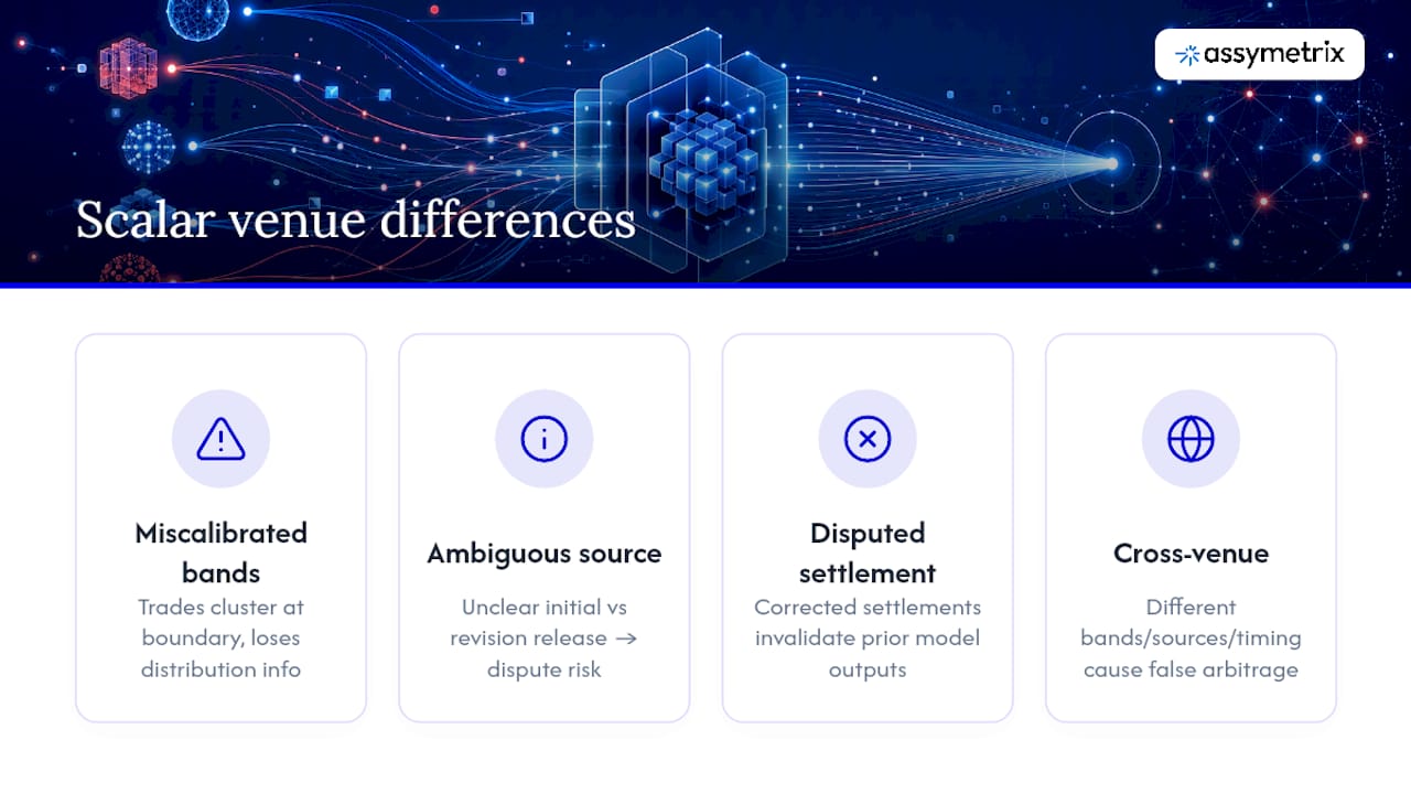
Miscalibrated bands are the most common practical headache. A venue sets a floor and cap based on historical volatility assumptions, and if those assumptions turn out wrong, most trading activity clusters near one boundary and the contract loses its informational value. Well-designed scalar markets calibrate their bounds so that most historical outcomes would have landed inside the range rather than pinned to an edge, which is precisely the design guidance that separates a useful scalar contract from a broken one. If you’re building a signal off a scalar market and the underlying value has spent the last six settlement cycles pinned near the cap, that market isn’t giving you distributional information anymore. It’s giving you a binary bet in scalar clothing.
Ambiguous resolution sources show up more often than you’d expect, especially on markets covering economic data with multiple possible reporting agencies or revision schedules. A contract that references “the official CPI print” without specifying whether that means the initial release or the first revision creates a genuine dispute risk, and venues handle these disputes with varying degrees of transparency. Some publish a clear appeals process with a bounded window; others leave settlement to an opaque internal review.
Disputed settlements are rare but consequential when they happen. A settlement value that gets challenged and later corrected invalidates any model output computed against the original figure, which is exactly why the revision-handling discipline described earlier in this piece isn’t optional if you’re running anything automated against these feeds.
Cross-venue normalization matters because the same underlying economic release or sports outcome often gets listed as a scalar market on more than one venue, sometimes with different bands, different resolution sources, and different settlement timing. Two venues might both list a market on quarterly GDP growth, but one settles off the Bureau of Economic Analysis’s advance estimate and the other waits for the second revision. Treating those two contracts as interchangeable in a cross-venue arbitrage model without accounting for the timing gap will generate false signals, because the price divergence you’re seeing might reflect a real information timing difference, not a mispricing.
This is the exact problem that pushes institutional trading infrastructure toward normalized schemas: venue-native data formats obscure real signals like arbitrage opportunities or coordinated smart-money movement unless you rebuild a common schema underneath them. A trader running a cross-venue strategy without that normalization layer is comparing apples to oranges and calling the difference alpha.
Practical rule of thumb for anyone building a venue-agnostic pipeline: pull the full contract spec text at ingestion time and store it alongside the market metadata, not just the current price. Specs change, get clarified, or get quietly updated after a dispute, and you want the version that was live when you took a position, not just whatever the venue shows today.
How Do You Build an Integration Pipeline for Scalar Market Data?
A production pipeline for scalar market data follows roughly six stages, and skipping any one of them tends to surface as a silent data quality problem weeks later rather than an obvious crash.
Hybrid ingestion. Combine REST snapshots for full order-book state on a polling interval with a websocket stream for real-time tick updates, and apply dedup rules keyed on a composite of market_id and timestamp so you don’t double-count a tick that arrives through both channels.
Validation checks. Before anything downstream touches the data, confirm floor is strictly less than cap, confirm a resolution source is present and non-null for any market approaching expiry, and run basic numeric sanity checks (no negative variance, no probability-like fields outside [0,1] where they’re supposed to be bounded).
Normalization. Apply the unit conversions, band rebasing, and timestamp canonicalization described earlier so every venue’s output lands in one consistent schema.
Enrichment. Compute derived fields, implied mean, implied variance, and any smart-money or wallet-tracking signals your models depend on, as a separate enrichment layer that sits on top of the normalized raw data rather than overwriting it.
Storage. Route high-frequency tick data to a time-series database for fast range queries, route aggregated market-level snapshots to an OLAP store for analytical queries, and archive raw venue payloads separately for reconciliation and audit.
Reconciliation testing. Periodically replay historical settlements through your normalization logic and confirm the output matches known-good values.
That last step deserves its own callout, because it’s the one most teams skip until something breaks in production.
Pro Tip: Build a “clamp test” into your CI pipeline that replays historical settlements against your current normalization logic before every deploy. Off-by-one decimal errors and unit-conversion bugs in clamp logic are quiet failures. They don’t throw exceptions. They just silently misprice every trade near a boundary until someone notices the P&L doesn’t add up.
Storage architecture decisions compound over time in ways that are hard to reverse cheaply. A time-series database like TimescaleDB or InfluxDB handles the tick-level write volume well, but analytical queries across thousands of markets for backtesting purposes usually run faster against a columnar OLAP layer. Keeping raw venue payloads in cheap object storage, untouched by any transformation, gives you a permanent audit trail you’ll be grateful for the first time a settlement dispute forces you to prove what a market actually showed at a specific timestamp.
Which Quant and AI Workflows Actually Benefit From Scalar Data?
Range-based quantitative strategies are the most direct use case: a trader with a view that a metric will land in the middle third of a published band, rather than at either extreme, can express that view directly through a scalar contract in a way no binary market allows. Binary markets force you to pick a single threshold and bet on either side of it. Scalar contracts let you express a genuinely distributional view, which maps far more naturally onto how quants already think about forecasting economic or sports outcomes.
Distribution fitting and belief-volatility surface construction turn a handful of scalar contracts on the same underlying event into something resembling an options chain. Once you have implied mean and variance across several strike bands, you can fit a full distribution and track how that distribution’s shape moves over time, the same way an options desk tracks implied volatility skew.
AI agents get a genuinely different input signal from scalar data than from binary data. A binary probability is a single scalar between 0 and 1, useful but informationally thin. A scalar market’s implied distribution gives an agent a continuous reward signal it can condition further decisions on, feed into an ensemble forecast alongside other model outputs, or use as a calibration check against its own internal probability estimates.
Cross-venue arbitrage between a scalar contract and a related binary contract on the same underlying event (a scalar band on GDP growth vs. a binary “will GDP exceed 2%” contract) can reveal pricing inconsistencies that a purely binary-to-binary comparison would miss entirely.
Economic indicator forecasting benefits directly from scalar data because magnitude genuinely matters for series like CPI, payrolls, or GDP growth, where “how much” carries far more decision-relevant information than a simple threshold crossing.
Ensemble forecasting pipelines can weight scalar-derived distributions alongside traditional econometric models, treating the market-implied distribution as one more input rather than a replacement for existing forecasting infrastructure.
How Does Assymetrix Normalize Scalar and Binary Prediction Market Data?
Assymetrix’s Data API returns scalar and binary market data through the same normalized schema, so a developer querying a scalar contract on Polymarket and a binary contract on Kalshi gets consistent field names, consistent timestamp formatting, and consistent provenance metadata back from a single integration. That matters because building three separate parsers for three venues (Polymarket, Kalshi, and Limitless) is exactly the kind of maintenance burden that breaks under its own weight the first time one venue changes its response format without notice.
A typical schema exposes fields such as floor, cap, resolution_value, resolution_time, implied_mean, implied_variance, and raw_tick alongside provenance fields that identify the resolution source and flag confidence level. Clamp logic, revision handling, and settlement hierarchy should be applied consistently before data reaches a developer’s application, rather than left as an exercise for every team that pulls the feed.
Scale gives that normalization work practical weight. A platform built on approximately 1.5 terabytes of historical data spanning nearly one billion rows of trading activity across major prediction market venues can provide enough depth to backtest clamp behavior, revision frequency, and band-calibration quality across thousands of historical scalar and binary contracts rather than a handful of recent examples.
Smart Money tracking surfaces wallet-level and account-level activity patterns correlated with historically accurate positioning, layered on top of the normalized data.
Trader Skill Scores rank market participants by demonstrated forecasting accuracy over time, giving quants a signal beyond raw price.
Cross-venue arbitrage signals flag pricing divergence between equivalent or related contracts across the three supported venues.
Historical coverage spans nearly a billion rows, enough to backtest normalization logic and clamp behavior against real settlement history rather than synthetic data.
Developer documentation and integration examples, including a Python-specific guide, are available for teams that want to see the schema in practice before committing engineering time to a full build.
What Should You Watch for When Backtesting Scalar Strategies?
Backtesting a scalar strategy on anything other than final settlement values, with the clamp formula applied consistently, produces numbers that look better in a spreadsheet than they will in live trading. The discipline here is narrower than it sounds, but the failure modes are common enough to name explicitly.
Backtest exclusively on final settlement values, applying the same clamp logic your production system uses. Testing against interim or unclamped values overstates edge near the boundaries.
Treat revision risk as a first-class model input, not an afterthought. If a series you’re trading revises meaningfully after initial release, your backtest needs to reflect that revision lag, not just the final number.
Avoid naive discretization of continuous outcomes into a handful of buckets for modeling convenience. Stress-test specifically against scenarios where the settlement value lands near the floor or cap, because that’s where clamp-driven nonlinearity does the most damage to a naive linear model.
Monitor book depth and execution impact before sizing a live strategy. Scalar markets frequently carry thinner liquidity than their binary counterparts on the same underlying event, and a backtest that assumes frictionless fills at the mid price will overstate real-world returns.
Pro Tip: Run a dedicated “boundary stress test” as a standing part of your backtest suite: isolate every historical settlement that landed within 5% of the floor or cap and check your model’s P&L attribution specifically in that subset. If performance looks dramatically different there than in the middle of the band, your model is quietly relying on clamp behavior it doesn’t actually understand.
Author Perspective: What Comes Next for Scalar Markets
Scalar markets won’t replace binary markets, and treating them as a competing product misreads what each contract type is good for. Binary markets answer discrete questions cheaply. Scalar markets carry magnitude, which is exactly the information a binary yes/no contract throws away. The two are complementary infrastructure for anyone trying to forecast a continuous variable.
What will determine whether scalar markets grow past their current niche is not clever contract design. It’s boring infrastructure: published settlement hierarchies, documented contract specs, and reproducible data pipelines that let a researcher trust a historical dataset without re-deriving it from raw venue archives. Institutional capital moves toward markets it can audit. Every unclamped payout, every ambiguous resolution source, every silent revision is a reason for that capital to stay on the sidelines a little longer.
— Dean
Get Normalized Scalar and Binary Data Through One Integration
Building three separate parsers for Polymarket, Kalshi, and Limitless costs engineering time that never shows up on a roadmap until it’s overdue. Assymetrix collapses that work into a single integration: normalized scalar and binary schemas, consistent clamp and provenance handling, and cross-venue Smart Money and arbitrage signals delivered through one Data API.
The API covers real-time and historical coverage across all three venues, backed by roughly 1.5 terabytes of historical trading data and nearly one billion rows spanning Polymarket, Kalshi, and Limitless. If you’re currently reconciling three venue-native formats by hand, that’s exactly the friction this API is built to remove. Start with the developer guide for integration examples, check the Python quickstart for working code samples, or review the accuracy benchmarks if you want to see how normalized data holds up against raw venue feeds before you commit engineering time. Request an API key and get a normalized scalar market feed running against real historical data within an afternoon.
Sources
For deeper technical grounding on the concepts covered here, consult the contract mechanics breakdown at NexusFi for clamp payoff derivations, the unified kernel paper on prediction market microstructure for belief-volatility surface construction, and Ravariant Labs’ research on scalar contract design for band calibration guidance. For the regulatory and institutionalization angle, see Katten’s analysis of event contract growth, and for market-level context on where scalar contracts fit into overall prediction market growth, see the LSE Business Review piece on tradable uncertainty.
Binary vs Scalar Prediction Markets: Different Contract Structures Explained
Toward Black–Scholes for Prediction Markets: A Unified Kernel and Market-Maker’s Handbook
Prediction markets have made uncertainty itself a tradable asset - LSE Business Review
FAQ
What Is Scalar Market Data in Prediction Markets?
Scalar market data covers numeric-outcome contracts that settle proportionally within a floor and cap using a clamp payoff formula, rather than resolving to a simple yes or no.
How Does a Scalar Payout Formula Work?
The payout equals (actual − floor) / (cap − floor), clamped between 0 and 1, meaning values outside the band pin to either 0 or 1 regardless of how far outside they landed.
Why Is Scalar Data Harder to Model Than Binary Data?
Scalar prices reflect an expected value inside a range rather than a single probability, so extracting a usable signal requires distributional modeling, revision handling, and clamp-aware backtesting instead of tracking one probability number.
Which Venues Offer Scalar or Range Prediction Markets?
Polymarket, Kalshi, and Limitless each list scalar or range-style contracts alongside binary markets, and each publishes its own floor, cap, and settlement rules that require normalization before cross-venue comparison.
Does Assymetrix Provide Normalized Scalar Market Data?
Yes. The Assymetrix Data API delivers normalized scalar and binary schemas across Polymarket, Kalshi, and Limitless through one integration, backed by roughly 1.5 terabytes of historical trading data.
Normalize Scalar Market Data for Devs & Quants, No Multiple Parsers
Scalar market data represents numeric-outcome event contracts whose payout equals a clamped linear mapping of a settled benchmark, not a single probability estimate. That distinction changes everything about how you ingest, model, and trade the data: a scalar tick is a point sample from an implied distribution, and treating it like a binary “yes” price will corrupt your backtests. The immediate implication for developers and quants is straightforward: normalize the schema, verify the resolution source, and model the outcome as a range before you write a single line of strategy code.
TL;DR:
Scalar market data reflects an expected value within a defined range using a clamped payoff formula, requiring careful normalization and handling of out-of-range settlements.
Accurate modeling demands incorporating distributional aspects, out-of-bound clamp risks, revision processes, and real-time streaming constraints.
Cross-venue normalization of contract specifications, resolution sources, and settlement details is essential to prevent misleading signals and enable reliable analysis.
Backtesting should focus on final settlement values with consistent clamp logic, treating revisions as noisy signals, and stress-testing near boundaries to avoid overestimating performance.
A unified data API that standardizes scalar and binary formats across multiple venues significantly reduces engineering overhead and improves data reliability for quantitative and AI workflows.
Assymetrixassymetrix.comNormalize Market Data OnceAssymetrix gives developers and quants unified scalar and binary prediction market data across Polymarket, Kalshi, and Limitless.Explore the data platform
Table of Contents
What Is a Scalar Prediction Market, and How Does It Differ From Binary?
Why Is Scalar Market Data Harder to Model Than Binary Data?
What Schema Fields Does a Scalar Market API Need to Return?
How Do Different Prediction Market Venues Publish Scalar Data?
How Do You Build an Integration Pipeline for Scalar Market Data?
Which Quant and AI Workflows Actually Benefit From Scalar Data?
How Does Assymetrix Normalize Scalar and Binary Prediction Market Data?
What Should You Watch for When Backtesting Scalar Strategies?
Author Perspective: What Comes Next for Scalar Markets
Get Normalized Scalar and Binary Data Through One Integration
Sources
What Is a Scalar Prediction Market, and How Does It Differ From Binary?
A scalar prediction market settles on a numeric value inside a defined range, and the contract pays out proportionally to where that value lands. A binary market resolves to one of two states, “yes” or “no,” and the payout is all or nothing. A scalar market on, say, next quarter’s inflation print doesn’t ask “will inflation exceed 3%?” It asks “where within a 0% to 6% band will inflation actually land?” and pays traders according to that position.
The math behind this is the clamp payoff formula, and every scalar contract you’ll encounter in the wild follows some version of it:
payout = clamp((actual − floor) / (cap − floor), 0, 1)
Three variables define the contract: the floor (the lowest value the market recognizes), the cap (the highest), and the settlement value (the actual observed outcome at resolution). If the settlement value lands below the floor or above the cap, the payout clamps to 0 or 1 respectively, which is why scalar contracts require special handling of out-of-range settlement that binary contracts never need to worry about.
Here’s the mechanics broken down for a working example. Say a scalar market on US nonfarm payrolls has a floor of 100,000 and a cap of 300,000. If the actual print comes in at 200,000, the payout calculates as (200,000 − 100,000) / (300,000 − 100,000) = 0.5. A print of 350,000 clamps to 1.0 even though it exceeds the cap by 50,000. A print of 50,000 clamps to 0 despite being 50,000 below the floor. Those clamps are not edge cases you can ignore. They are structural features of the contract that determine your P&L at the boundaries.
Binary markets skip all of this. A binary contract on “will the Fed cut rates in March” resolves to exactly 1 or 0 based on a single triggering event. There’s no floor, no cap, no proportional mapping. The price you observe before resolution is a probability estimate; the price a scalar market shows you before resolution is closer to an expected value of the underlying metric within the band, which is a fundamentally different statistical object to model.
Resolution mechanics matter as much as the payoff formula, and this is where a lot of naive integrations break:
Resolution source: every contract spec names an authoritative data provider (a government statistics bureau, an index provider, a specific exchange feed) and the venue’s smart contract or settlement engine reads from that source alone.
Revision rules: many economic series get revised after initial release. A contract spec should state whether it settles on the first print or a revised figure, and when.
Dispute windows: some venues hold a challenge period after initial settlement during which a result can be contested and corrected.
Precision and rounding: contract specs typically define the decimal precision used for both the floor/cap band and the final settlement comparison.
Miss any one of these four items when parsing a contract spec, and you’ll misattribute a settlement value, misclamp a payout, or trust a print that later gets revised out from under you.
Why Is Scalar Market Data Harder to Model Than Binary Data?
Binary market data gives you one number to track: an implied probability that moves between 0 and 1. Scalar market data gives you a price that represents where the market thinks the expected value sits inside a band, and extracting anything useful from that requires modeling an entire implied distribution, not a single scalar (the irony of the naming isn’t lost on anyone who works with this data daily).
The core challenge breaks into four distinct problems:
Distributional modeling, not probability estimation. A scalar price embeds information about the mean of the underlying distribution, but says nothing directly about variance, skew, or tail risk. Extracting a full belief distribution from a handful of scalar contracts at different strikes on the same underlying event requires curve-fitting techniques closer to options-market implied volatility surfaces than anything in classic binary forecasting.
Clamp and jump risk at expiry. Because payouts clamp at the boundaries, a market trading near the floor or cap behaves nonlinearly as expiry approaches. A settlement value that jumps just past the cap produces a discontinuous payoff, and if your backtest doesn’t model that discontinuity explicitly, you’ll systematically overstate or understate strategy returns near the boundaries.
Revision handling. Initial economic prints get revised, sometimes materially. A pipeline that treats the first settlement print as final will mislabel training data for any model trained on historical outcomes. The safer approach treats every initial print as a noisy, time-stamped observation, not ground truth.
Latency and streaming constraints. High-frequency agents trading scalar markets need sub-second visibility into order book changes, not just periodic snapshots, because scalar markets often have thinner liquidity than headline binary markets on the same underlying event and price discovery can be choppier.
Academic work on prediction market microstructure backs this up directly. A unified stochastic kernel approach to prediction markets proposes treating traded probabilities as martingales and building a calibration pipeline that filters microstructure noise before you can extract belief-volatility or jump-intensity surfaces. Skip that filtering step, and your “distribution” is mostly noise dressed up as signal.
Pro Tip: Never train a model directly on raw scalar ticks. Run them through a denoising or smoothing pass first, and keep both the raw and the smoothed series in storage. You will eventually need to explain a divergence between the two, and reconstructing the raw feed after the fact is far harder than storing it up front.
The revision problem deserves one more sentence of emphasis: treat every initial settlement print as a noisy, time-stamped observation rather than a final value, and compute both a point estimate and a smoothed distribution per market window for anything downstream that depends on it, a pattern borne out in recent kernel-based modeling work on prediction markets.
What Schema Fields Does a Scalar Market API Need to Return?
A production-grade scalar data feed needs a canonical schema that survives contact with three or more venues, each with its own idiosyncratic contract naming and settlement logic. The fields below represent the minimum viable schema for any pipeline that wants to run models across scalar markets without venue-specific branching logic scattered through the codebase.
event_id / market_id: stable identifiers that persist across venue-side renames or contract relistings.
floor / cap: the numeric bounds of the contract, normalized to a consistent unit (see below).
resolution_value: the final settled numeric outcome, populated only after settlement.
resolution_time: the timestamp of final settlement, distinct from the market’s close time.
implied_mean / implied_variance: derived fields computed from the current order book, not raw venue output.
raw_tick: the unmodified price as reported by the venue, preserved for audit and reconciliation.
provenance fields: resolution source URL, data provider name, and a confidence flag.
Normalization is where most of the real engineering work happens. Unit and scale conversion matters because one venue might quote a market in raw index points while another quotes the same underlying series as a percentage change. Band rebasing matters because two venues covering the same economic release sometimes choose different floor/cap ranges for what is nominally the same event, and comparing them without rebasing to a common scale produces meaningless deltas. Timestamp canonicalization matters because venues report in different time zones and precision levels, and clamp enforcement matters because you need to apply the payout formula consistently even when a venue’s own UI doesn’t show you the clamped value directly.
Quality flags close the loop on auditability. A schema should expose is_revised (whether the resolution value has changed since first reported), resolution_confidence (a categorical or numeric flag reflecting how authoritative the current settlement value is), and a provenance_url pointing to the source document or feed the settlement was drawn from. Exposing those three flags in streaming payloads lets live trading agents alter behavior the moment a market’s resolution confidence drops, rather than discovering the problem after a bad fill.
How Do Different Prediction Market Venues Publish Scalar Data?
Every venue that lists scalar or range contracts publishes its own version of the contract spec, and the differences between them are exactly where naive ingestion pipelines tend to break. Three pieces of metadata show up on nearly every venue’s spec page: the floor and cap values, the settlement rule (which data source and which specific release the contract references), and the decimal precision used for both the band and the final comparison. Beyond that baseline, the idiosyncrasies start piling up.
Miscalibrated bands are the most common practical headache. A venue sets a floor and cap based on historical volatility assumptions, and if those assumptions turn out wrong, most trading activity clusters near one boundary and the contract loses its informational value. Well-designed scalar markets calibrate their bounds so that most historical outcomes would have landed inside the range rather than pinned to an edge, which is precisely the design guidance that separates a useful scalar contract from a broken one. If you’re building a signal off a scalar market and the underlying value has spent the last six settlement cycles pinned near the cap, that market isn’t giving you distributional information anymore. It’s giving you a binary bet in scalar clothing.
Ambiguous resolution sources show up more often than you’d expect, especially on markets covering economic data with multiple possible reporting agencies or revision schedules. A contract that references “the official CPI print” without specifying whether that means the initial release or the first revision creates a genuine dispute risk, and venues handle these disputes with varying degrees of transparency. Some publish a clear appeals process with a bounded window; others leave settlement to an opaque internal review.
Disputed settlements are rare but consequential when they happen. A settlement value that gets challenged and later corrected invalidates any model output computed against the original figure, which is exactly why the revision-handling discipline described earlier in this piece isn’t optional if you’re running anything automated against these feeds.
Cross-venue normalization matters because the same underlying economic release or sports outcome often gets listed as a scalar market on more than one venue, sometimes with different bands, different resolution sources, and different settlement timing. Two venues might both list a market on quarterly GDP growth, but one settles off the Bureau of Economic Analysis’s advance estimate and the other waits for the second revision. Treating those two contracts as interchangeable in a cross-venue arbitrage model without accounting for the timing gap will generate false signals, because the price divergence you’re seeing might reflect a real information timing difference, not a mispricing.
This is the exact problem that pushes institutional trading infrastructure toward normalized schemas: venue-native data formats obscure real signals like arbitrage opportunities or coordinated smart-money movement unless you rebuild a common schema underneath them. A trader running a cross-venue strategy without that normalization layer is comparing apples to oranges and calling the difference alpha.
Practical rule of thumb for anyone building a venue-agnostic pipeline: pull the full contract spec text at ingestion time and store it alongside the market metadata, not just the current price. Specs change, get clarified, or get quietly updated after a dispute, and you want the version that was live when you took a position, not just whatever the venue shows today.
How Do You Build an Integration Pipeline for Scalar Market Data?
A production pipeline for scalar market data follows roughly six stages, and skipping any one of them tends to surface as a silent data quality problem weeks later rather than an obvious crash.
Hybrid ingestion. Combine REST snapshots for full order-book state on a polling interval with a websocket stream for real-time tick updates, and apply dedup rules keyed on a composite of market_id and timestamp so you don’t double-count a tick that arrives through both channels.
Validation checks. Before anything downstream touches the data, confirm floor is strictly less than cap, confirm a resolution source is present and non-null for any market approaching expiry, and run basic numeric sanity checks (no negative variance, no probability-like fields outside [0,1] where they’re supposed to be bounded).
Normalization. Apply the unit conversions, band rebasing, and timestamp canonicalization described earlier so every venue’s output lands in one consistent schema.
Enrichment. Compute derived fields, implied mean, implied variance, and any smart-money or wallet-tracking signals your models depend on, as a separate enrichment layer that sits on top of the normalized raw data rather than overwriting it.
Storage. Route high-frequency tick data to a time-series database for fast range queries, route aggregated market-level snapshots to an OLAP store for analytical queries, and archive raw venue payloads separately for reconciliation and audit.
Reconciliation testing. Periodically replay historical settlements through your normalization logic and confirm the output matches known-good values.
That last step deserves its own callout, because it’s the one most teams skip until something breaks in production.
Pro Tip: Build a “clamp test” into your CI pipeline that replays historical settlements against your current normalization logic before every deploy. Off-by-one decimal errors and unit-conversion bugs in clamp logic are quiet failures. They don’t throw exceptions. They just silently misprice every trade near a boundary until someone notices the P&L doesn’t add up.
Storage architecture decisions compound over time in ways that are hard to reverse cheaply. A time-series database like TimescaleDB or InfluxDB handles the tick-level write volume well, but analytical queries across thousands of markets for backtesting purposes usually run faster against a columnar OLAP layer. Keeping raw venue payloads in cheap object storage, untouched by any transformation, gives you a permanent audit trail you’ll be grateful for the first time a settlement dispute forces you to prove what a market actually showed at a specific timestamp.
Which Quant and AI Workflows Actually Benefit From Scalar Data?
Range-based quantitative strategies are the most direct use case: a trader with a view that a metric will land in the middle third of a published band, rather than at either extreme, can express that view directly through a scalar contract in a way no binary market allows. Binary markets force you to pick a single threshold and bet on either side of it. Scalar contracts let you express a genuinely distributional view, which maps far more naturally onto how quants already think about forecasting economic or sports outcomes.
Distribution fitting and belief-volatility surface construction turn a handful of scalar contracts on the same underlying event into something resembling an options chain. Once you have implied mean and variance across several strike bands, you can fit a full distribution and track how that distribution’s shape moves over time, the same way an options desk tracks implied volatility skew.
AI agents get a genuinely different input signal from scalar data than from binary data. A binary probability is a single scalar between 0 and 1, useful but informationally thin. A scalar market’s implied distribution gives an agent a continuous reward signal it can condition further decisions on, feed into an ensemble forecast alongside other model outputs, or use as a calibration check against its own internal probability estimates.
Cross-venue arbitrage between a scalar contract and a related binary contract on the same underlying event (a scalar band on GDP growth vs. a binary “will GDP exceed 2%” contract) can reveal pricing inconsistencies that a purely binary-to-binary comparison would miss entirely.
Economic indicator forecasting benefits directly from scalar data because magnitude genuinely matters for series like CPI, payrolls, or GDP growth, where “how much” carries far more decision-relevant information than a simple threshold crossing.
Ensemble forecasting pipelines can weight scalar-derived distributions alongside traditional econometric models, treating the market-implied distribution as one more input rather than a replacement for existing forecasting infrastructure.
How Does Assymetrix Normalize Scalar and Binary Prediction Market Data?
Assymetrix’s Data API returns scalar and binary market data through the same normalized schema, so a developer querying a scalar contract on Polymarket and a binary contract on Kalshi gets consistent field names, consistent timestamp formatting, and consistent provenance metadata back from a single integration. That matters because building three separate parsers for three venues (Polymarket, Kalshi, and Limitless) is exactly the kind of maintenance burden that breaks under its own weight the first time one venue changes its response format without notice.
A typical schema exposes fields such as floor, cap, resolution_value, resolution_time, implied_mean, implied_variance, and raw_tick alongside provenance fields that identify the resolution source and flag confidence level. Clamp logic, revision handling, and settlement hierarchy should be applied consistently before data reaches a developer’s application, rather than left as an exercise for every team that pulls the feed.
Scale gives that normalization work practical weight. A platform built on approximately 1.5 terabytes of historical data spanning nearly one billion rows of trading activity across major prediction market venues can provide enough depth to backtest clamp behavior, revision frequency, and band-calibration quality across thousands of historical scalar and binary contracts rather than a handful of recent examples.
Smart Money tracking surfaces wallet-level and account-level activity patterns correlated with historically accurate positioning, layered on top of the normalized data.
Trader Skill Scores rank market participants by demonstrated forecasting accuracy over time, giving quants a signal beyond raw price.
Cross-venue arbitrage signals flag pricing divergence between equivalent or related contracts across the three supported venues.
Historical coverage spans nearly a billion rows, enough to backtest normalization logic and clamp behavior against real settlement history rather than synthetic data.
Developer documentation and integration examples, including a Python-specific guide, are available for teams that want to see the schema in practice before committing engineering time to a full build.
What Should You Watch for When Backtesting Scalar Strategies?
Backtesting a scalar strategy on anything other than final settlement values, with the clamp formula applied consistently, produces numbers that look better in a spreadsheet than they will in live trading. The discipline here is narrower than it sounds, but the failure modes are common enough to name explicitly.
Backtest exclusively on final settlement values, applying the same clamp logic your production system uses. Testing against interim or unclamped values overstates edge near the boundaries.
Treat revision risk as a first-class model input, not an afterthought. If a series you’re trading revises meaningfully after initial release, your backtest needs to reflect that revision lag, not just the final number.
Avoid naive discretization of continuous outcomes into a handful of buckets for modeling convenience. Stress-test specifically against scenarios where the settlement value lands near the floor or cap, because that’s where clamp-driven nonlinearity does the most damage to a naive linear model.
Monitor book depth and execution impact before sizing a live strategy. Scalar markets frequently carry thinner liquidity than their binary counterparts on the same underlying event, and a backtest that assumes frictionless fills at the mid price will overstate real-world returns.
Pro Tip: Run a dedicated “boundary stress test” as a standing part of your backtest suite: isolate every historical settlement that landed within 5% of the floor or cap and check your model’s P&L attribution specifically in that subset. If performance looks dramatically different there than in the middle of the band, your model is quietly relying on clamp behavior it doesn’t actually understand.
Author Perspective: What Comes Next for Scalar Markets
Scalar markets won’t replace binary markets, and treating them as a competing product misreads what each contract type is good for. Binary markets answer discrete questions cheaply. Scalar markets carry magnitude, which is exactly the information a binary yes/no contract throws away. The two are complementary infrastructure for anyone trying to forecast a continuous variable.
What will determine whether scalar markets grow past their current niche is not clever contract design. It’s boring infrastructure: published settlement hierarchies, documented contract specs, and reproducible data pipelines that let a researcher trust a historical dataset without re-deriving it from raw venue archives. Institutional capital moves toward markets it can audit. Every unclamped payout, every ambiguous resolution source, every silent revision is a reason for that capital to stay on the sidelines a little longer.
— Dean
Get Normalized Scalar and Binary Data Through One Integration
Building three separate parsers for Polymarket, Kalshi, and Limitless costs engineering time that never shows up on a roadmap until it’s overdue. Assymetrix collapses that work into a single integration: normalized scalar and binary schemas, consistent clamp and provenance handling, and cross-venue Smart Money and arbitrage signals delivered through one Data API.
The API covers real-time and historical coverage across all three venues, backed by roughly 1.5 terabytes of historical trading data and nearly one billion rows spanning Polymarket, Kalshi, and Limitless. If you’re currently reconciling three venue-native formats by hand, that’s exactly the friction this API is built to remove. Start with the developer guide for integration examples, check the Python quickstart for working code samples, or review the accuracy benchmarks if you want to see how normalized data holds up against raw venue feeds before you commit engineering time. Request an API key and get a normalized scalar market feed running against real historical data within an afternoon.
Sources
For deeper technical grounding on the concepts covered here, consult the contract mechanics breakdown at NexusFi for clamp payoff derivations, the unified kernel paper on prediction market microstructure for belief-volatility surface construction, and Ravariant Labs’ research on scalar contract design for band calibration guidance. For the regulatory and institutionalization angle, see Katten’s analysis of event contract growth, and for market-level context on where scalar contracts fit into overall prediction market growth, see the LSE Business Review piece on tradable uncertainty.
Binary vs Scalar Prediction Markets: Different Contract Structures Explained
Toward Black–Scholes for Prediction Markets: A Unified Kernel and Market-Maker’s Handbook
Prediction markets have made uncertainty itself a tradable asset - LSE Business Review
FAQ
What Is Scalar Market Data in Prediction Markets?
Scalar market data covers numeric-outcome contracts that settle proportionally within a floor and cap using a clamp payoff formula, rather than resolving to a simple yes or no.
How Does a Scalar Payout Formula Work?
The payout equals (actual − floor) / (cap − floor), clamped between 0 and 1, meaning values outside the band pin to either 0 or 1 regardless of how far outside they landed.
Why Is Scalar Data Harder to Model Than Binary Data?
Scalar prices reflect an expected value inside a range rather than a single probability, so extracting a usable signal requires distributional modeling, revision handling, and clamp-aware backtesting instead of tracking one probability number.
Which Venues Offer Scalar or Range Prediction Markets?
Polymarket, Kalshi, and Limitless each list scalar or range-style contracts alongside binary markets, and each publishes its own floor, cap, and settlement rules that require normalization before cross-venue comparison.
Does Assymetrix Provide Normalized Scalar Market Data?
Yes. The Assymetrix Data API delivers normalized scalar and binary schemas across Polymarket, Kalshi, and Limitless through one integration, backed by roughly 1.5 terabytes of historical trading data.
Other Blog


