3 Proper Scoring Rules Researchers and Market Quants Must Use
3 Proper Scoring Rules Researchers and Market Quants Must Use
3 Proper Scoring Rules Researchers and Market Quants Must Use
Research explainer of proper scoring rules: when to use log score, Brier, or CRPS, plus 2024–2026 findings and effects on model training.

3 Proper Scoring Rules Researchers and Market Quants Must Use
A scoring rule assigns a numeric score to a probabilistic forecast once the outcome is known, and it is proper when reporting the true predictive distribution optimizes the expected score, strictly proper when that optimum is unique. For researchers, the practical rule is simple: match the score to the forecast object, whether that is a pmf, a density, a CDF, or a quantile, then use that same proper rule for both evaluation and training. The three workhorses are the logarithmic score, the Brier (quadratic) score, and the continuous ranked probability score, each suited to a different forecast shape.
TL;DR:
The proper scoring rule must match the forecast object, such as density or quantile, to ensure unbiased evaluation and training.
The logarithmic score is best for likelihood-based models and is highly sensitive to overconfidence by penalizing tiny probabilities assigned to realized outcomes.
CRPS is ideal for ensemble and continuous forecasts, rewarding predictions close to the outcome without explosion near zero probabilities, and can be computed from samples.
Brier scores are suitable for categorical forecasts, providing bounded, interpretable calibration metrics and decomposing prediction quality into calibration and resolution.
Implementation accuracy requires consistent orientation, correct forecast object matching, and avoiding smoothing or post-processing that breaks propriety guarantees.
AssymetrixBring Market Data Into Your ModelsAssymetrix unifies prediction market data across Polymarket, Kalshi, and Limitless through one integration for research and trading tools.Explore Assymetrix
Table of Contents
Definitions and core properties of scoring rules
Common scoring rules: formulas, scope, and intuition
Mathematical foundations: entropy, Bregman divergences, and representations
How to choose a scoring rule for evaluation or training
Using scoring rules for estimation and model training
Computation, implementation notes, and pitfalls to avoid
Recent research and empirical comparisons (2024–2026): what changed and open questions
Implications for prediction-market engineers and quant teams
Sources
Definitions and core properties of scoring rules
A scoring rule is a function S(P, y) that takes a forecaster’s predictive distribution P and a realized outcome y and returns a number. Depending on convention, that number is a reward to maximize or a loss to minimize. It helps to define the expected score, S(P, Q), as the expected value of S(P, y) when y is drawn from the true distribution Q. This separates the forecast actually issued (P) from the distribution nature actually uses to generate outcomes (Q), which is exactly the distinction that propriety is built on.
A scoring rule is proper relative to a class of distributions when, for every true distribution Q in that class, the expected score S(P, Q) is optimized by setting P equal to Q. In plain terms: no other forecast beats telling the truth, in expectation. It is strictly proper when Q is the unique optimizer, so that no distinct distribution can tie the truth-telling forecast. The formal characterization from Gneiting and Raftery covers this across categorical probabilities, predictive densities, CDFs, quantiles, and intervals, which is why the framework generalizes so cleanly across forecast types.
Underneath this definition sits a convexity condition. The expected score, viewed as a function of the reported distribution, behaves like a concave entropy functional, and propriety falls out of that concavity. Strict propriety corresponds to strict concavity, which is what forces the optimum to be unique rather than merely tied. This connection to entropy and convex analysis is why proper scoring rules show up in statistical decision theory, information theory, and elicitation theory as the same underlying object wearing different names.
Two practical conventions matter once you start implementing scores rather than just defining them:
Orientation: some rules are stated as rewards (higher is better) and others as losses (lower is better); affine transformations preserve propriety, but sign flips change which direction counts as “good,” so document orientation explicitly.
Sample aggregation: the expected score S(P, Q) is a theoretical quantity; in practice you compute a sample average of S(P, y) over realized outcomes, which converges to the expected score as sample size grows but carries finite-sample noise that matters for small backtests.
Scale invariance: because affine transformations of a proper score remain proper, two scores that differ only by a constant or a positive scaling factor rank forecasters identically, even though their raw numbers differ.
Forecast-object matching: a rule proper for densities is not automatically proper for quantile forecasts of the same quantity, so the object being scored has to match the object the rule was designed for.
These conventions are not cosmetic. A researcher who mixes orientation (treating a loss as a reward) or aggregates scores across mismatched forecast objects can produce model comparisons that look rigorous but are quietly broken.
Common scoring rules: formulas, scope, and intuition
Three rules account for most applied work, and each has a distinct personality.
The logarithmic score is defined as the negative log density or probability assigned to the realized outcome: for a discrete outcome y with predicted probability p(y), the loss form is −log p(y). It is strictly proper, and minimizing it over a parametric family is mathematically identical to maximum-likelihood estimation, which is why every likelihood-based model is, implicitly, being scored with the log rule. The log score is local, meaning it only depends on the probability mass or density assigned to the outcome that actually occurred, not on how probability is distributed elsewhere. That locality has a sharp edge: log score’s sensitivity to near-zero assigned probabilities means that a forecaster who assigns a tiny probability to an outcome that then occurs is penalized severely, since the loss blows up as p(y) approaches zero. This makes the log score an effective detector of overconfidence.
The Brier score, also called the quadratic score, was built for categorical and binary forecasts. For a binary outcome with predicted probability p and realized outcome y in {0, 1}, the Brier score is (p − y)². It generalizes to multi-category settings as a sum of squared differences between predicted and actual class indicators. Unlike the log score, Brier is bounded and does not explode near zero, which makes it more forgiving of confident misses and more directly interpretable as a calibration-plus-resolution decomposition: squared error that splits into how well-calibrated the forecaster is and how much the forecaster’s predictions vary across cases.
The continuous ranked probability score (CRPS) extends this logic to continuous outcomes. It integrates the squared difference between the forecaster’s predictive CDF and the step-function CDF of the realized observation, across the whole real line. The Gneiting and Raftery characterization confirms CRPS is proper, and strictly proper whenever the forecast distribution has finite first moment. When the forecast is a point mass, CRPS reduces exactly to absolute error, which gives it an intuitive anchor: it behaves like a distribution-aware generalization of the mean absolute error. CRPS is distance-sensitive: probability mass placed near the realized outcome is rewarded more than probability placed far away, even if both are technically “wrong.” That is a meaningful contrast with the log score’s locality, and it is also why CRPS is essentially the integral of the Brier score, an L2 distance between forecast and observation CDFs that exists for any distribution with a finite first moment. It is particularly convenient for ensemble forecasts, since it can be estimated directly from a sample of ensemble members without needing a closed-form density.
Beyond these three, several related families extend the toolkit:
Spherical and pseudospherical scores are local like the log score but use power transformations instead of a logarithm, giving a tunable sensitivity parameter.
Energy scores generalize CRPS to multivariate outcomes by replacing absolute difference with a vector norm between sampled forecast draws and the realized vector.
Kernel scores build proper rules from a choice of positive-definite kernel, with CRPS and the energy score as particular cases.
Matching the rule to the forecast object is the decision that matters most in practice. A categorical pmf calls for the Brier score or the log score in its discrete form. A continuous density calls for the log score evaluated at the observed value. A full predictive CDF, especially from an ensemble or simulation, calls for CRPS. A quantile or interval forecast needs a quantile-specific or interval-specific proper scoring rule such as the pinball loss, which is a different object from a density and should not be scored with CRPS or the log score directly.
Mathematical foundations: entropy, Bregman divergences, and representations
The theoretical backbone connecting all of this is a representation result: expected scores behave as concave, entropy-like functionals of the reported distribution, and propriety is the condition that this concave functional is optimized exactly at the truth. This is sometimes called a Savage representation, after the broader decision-theoretic result that any proper scoring rule can be derived from a convex function via a subgradient construction. The arXiv treatment of proper scoring rules for estimation and forecast evaluation lays out representation theorems showing the equivalence between propriety and concavity or convexity conditions, alongside kernel-score constructions that recover many standard examples.
This convexity link is not an abstraction researchers can ignore. It is the mechanism that produces Bregman divergences from scoring rules. Every strictly proper scoring rule has an associated divergence measuring the “distance” between the reported distribution and the true one, and that divergence is a Bregman divergence generated by the convex function underlying the score. The log score’s associated divergence is the Kullback-Leibler divergence, which is the special case most researchers already know by name, but the same construction works for any convex generator, producing a different divergence for each choice.
Kernel-score construction extends this further. Given a positive-definite kernel on the outcome space, there is a canonical way to build a strictly proper scoring rule from it, and CRPS and the energy score both arise as specific instances of this construction applied to different kernels. This is useful beyond theoretical tidiness: it means a researcher who needs a proper score for a multivariate or non-standard outcome space can often construct one directly from a suitable kernel rather than searching for a bespoke formula.
The practical payoff of all this machinery is a single implication worth holding onto: strict propriety is equivalent to strict convexity of the underlying generator, and strict convexity is what guarantees a unique optimum. Without strict convexity, you can end up with a scoring rule that is merely proper, where multiple distributions tie at the optimal expected score, which weakens its usefulness as an estimation target because gradient-based optimization has no single point to converge to.

How to choose a scoring rule for evaluation or training
Picking a score is a short decision process, not a matter of taste.
Identify the forecast object you actually have: a categorical probability vector, a predictive density, a full CDF, a quantile, or an interval. The score must be strictly consistent for that specific object, not merely “proper in general.”
Decide whether you care more about exposing overconfidence or about rewarding near-misses. The log score is local and penalizes overconfidence sharply near zero probability; CRPS is distance-sensitive and gives partial credit for probability mass placed close to, but not exactly on, the outcome.
Check whether your evaluation needs to handle ensembles or simulated draws rather than closed-form densities. CRPS is estimable directly from samples, which makes it a natural fit for ensemble-based or simulation-based forecasts.
Consider computational and robustness constraints. If your model has an intractable normalizing constant, a homogeneous or local scoring rule can sidestep that problem entirely, since it does not require evaluating the full normalized density.
Decide whether you need a composite or weighted score, for example when certain parts of the outcome space (tails, specific categories) matter more than others for your application.
The trade-offs compress into one line each: the log score is local and unforgiving of near-zero misses, which makes it a strong overconfidence detector; Brier is bounded and interpretable through calibration-resolution decomposition; CRPS is distance-aware and well-suited to continuous or ensemble forecasts where “close” should count for something.
Pro Tip: Before writing any evaluation code, state out loud which forecast object you are scoring; most propriety bugs come from silently switching between a density, a CDF, and a sample-based approximation mid-pipeline.
A short checklist before committing to a score: What object does your model actually output? Do you need the score for evaluation only, or also as a training loss? Does your data include ensembles or single point estimates? Is a normalizing constant tractable? Does the application care more about tail misses than about average distance?
Using scoring rules for estimation and model training
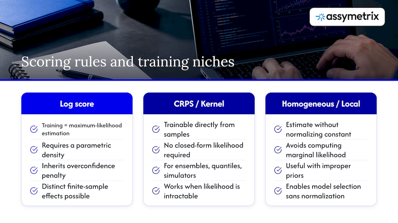
A scoring rule is a loss function the moment you minimize its sample average over model parameters, and this is where the theory connects directly to estimation practice. The clearest case is the log score: minimizing the sample average of −log p(y; θ) over θ is exactly maximum-likelihood estimation. Every time a researcher fits a parametric model by maximizing likelihood, that fit is, by construction, log-score minimization, inheriting all the properties, strengths, and the overconfidence penalty, that come with it.
CRPS and kernel scores extend this to distributional learners that do not output a simple parametric density. A model producing an ensemble of plausible outcomes, a quantile forecaster, or a simulation-based generative model can be trained by minimizing sample CRPS directly, since CRPS is computable from samples without requiring a closed-form likelihood. This matters for architectures where likelihood is intractable or undefined, where kernel and energy scores give a path to training that log-likelihood cannot.
Recent empirical work complicates the assumption that any strictly proper rule is interchangeable as a training objective. Experimental comparisons across strictly proper training rules found that different proper training objectives can produce distinct calibration and bias profiles in finite-sample ML training, with Brier-trained and log-trained models behaving differently even when both are theoretically unbiased in expectation. In one such experiment, the Brier-trained model achieved the lowest Brier score while the log-trained model achieved the lowest calibration error, a result the authors flag as dependent on single-seed experimental variability rather than a settled ranking. The practical lesson is that theoretical interchangeability of proper rules does not guarantee identical finite-sample behavior, so the choice of training objective should be validated empirically for the specific model and dataset rather than assumed from theory alone.
Score-based estimation also has a specific niche worth naming directly: situations with intractable normalizing constants. Homogeneous and local scoring rules let you estimate parameters and perform model selection without ever computing the normalizing constant, which makes them practical for Bayesian model comparison under improper priors, where the marginal likelihood is undefined or prohibitively expensive to compute.
Computation, implementation notes, and pitfalls to avoid
Computing CRPS in practice has two paths. When the predictive distribution has a closed form, such as a Gaussian or a known parametric family, CRPS has closed-form expressions in terms of that distribution’s CDF and density. When the forecast is an ensemble of samples, CRPS can be estimated directly from the sample, using the pairwise-distance formulation that avoids ever constructing an explicit CDF, which is one reason CRPS is popular for simulation-heavy forecasting pipelines.
Orientation conventions in software are a recurring source of silent bugs. The scikit-learn model evaluation documentation uses a higher-is-better convention for scorers, which means losses are frequently negated in naming, such as neg_log_loss, so that cross-validation routines that maximize a scorer still end up minimizing the underlying loss. Carrying an unnegated loss into a maximization routine, or vice versa, produces a model selection process that silently optimizes the wrong direction.
A short set of implementation habits avoids most of the damage:
Clip or floor predicted probabilities before taking a logarithm, since an exact zero probability assigned to an outcome that occurs produces an infinite log-score penalty.
Use log-sum-exp style numerically stable formulations when probabilities come from softmax outputs, to avoid underflow in very small probability regions.
Compute CRPS from samples only when the reported forecast object is genuinely a sample-based distribution, not a post-processed or smoothed version of one.
Document orientation (loss vs reward) at every stage of a pipeline that compares models across different scoring functions.
Pro Tip: Treat any smoothing step applied to a forecast before scoring as a change to the forecast object itself; scoring the smoothed output as if it were the original declared forecast is a quiet way to break propriety.
That last point deserves emphasis because it is easy to miss. Smoothing a submitted forecast before scoring it can destroy propriety unless the reporter’s declared forecast object matches the postprocessed object being scored. If a model reports raw ensemble members but the evaluation pipeline applies a kernel-density smoother before computing CRPS, the score no longer measures what the model actually reported, and the propriety guarantees no longer apply.
Recent research and empirical comparisons (2024–2026): what changed and open questions
Recent review work positions proper scoring rules as doing double duty: evaluators of forecast quality and estimators for model training, with the 2025 treatment of proper scoring rules for estimation and forecast evaluation framing both roles through the same entropy and kernel-score machinery described above. That dual framing matters because it means the same theoretical object that ranks forecasters in a leaderboard can, with minimal modification, become a training loss for the next model generation.
The more unsettled territory is empirical. The 2026 experimental comparison of strictly proper rules found that five strictly proper rules all incentivize truthful reporting in theory, yet produced measurably different calibration and bias profiles when actually used as training objectives, with the authors explicitly cautioning that results may be sensitive to single-seed experimental variability rather than representing a stable ranking across rules. Open questions that follow directly from this include how sensitive these differences are to sample size, whether tail behavior under different rules converges as data grows, and how computational cost scales when kernel or energy scores replace simpler closed-form losses in large training runs.
For practitioners, the honest takeaway is to treat theoretical propriety as a necessary condition for a sound training objective, not a sufficient one, and to validate finite-sample behavior with held-out calibration checks before committing to a rule for production model training.
Implications for prediction-market engineers and quant teams
Choosing a score is not an academic exercise when it feeds a trader-skill leaderboard or a Smart Money signal. A skill metric built on the log score will flag overconfident traders harshly for near-miss calls, while one built on CRPS will reward traders whose probability mass lands close to outcomes even when it is not exactly right, and those are different definitions of “good at forecasting” that will rank the same trader differently.
Backtests face the same choice. A cross-venue arbitrage signal evaluated with a mismatched scoring rule can look stronger or weaker than it actually is, simply because the scorer does not match the forecast object the signal produces. Computing these scores at scale requires distributional inputs across venues, which is the layer Assymetrix’s Data API is built to supply: normalized, cross-venue price and trade data from Polymarket, Kalshi, and Limitless that can feed directly into a scoring pipeline rather than a bespoke per-venue parser.
The practical note for model pipelines: pick the scoring rule before building the evaluation dashboard, not after, since the choice shapes which trades your backtest rewards; see this Probability Calibration Trading Guide for Traders for more on calibration and score selection.
— Dean
Sources
FAQ
What are scoring rules?
A scoring rule is a function that assigns a numerical score to a probabilistic forecast once the outcome it predicted is observed, used to evaluate or train forecasters. The rule is proper when the forecaster’s expected score is optimized by reporting the true distribution, which is the property that makes scoring rules useful for both evaluation and estimation, as formalized by Gneiting and Raftery.
How do you interpret a CRPS score?
CRPS measures the distance between a forecaster’s predictive CDF and the realized outcome by integrating squared CDF differences, and it reduces to plain absolute error for a point forecast. It is distance-sensitive, so probability mass placed near the eventual outcome scores better than mass placed far away, even when both forecasts miss the exact value, as described in the CRPS framework from Gneiting and Raftery.
What is a scoring procedure?
A scoring procedure is the practical process of applying a scoring rule: matching the rule to the forecast object (pmf, density, CDF, or quantile), computing the score for each realized outcome, and aggregating scores across a sample to compare forecasters or models. Getting the procedure right depends on consistent orientation (reward versus loss) and on scoring the forecast object exactly as it was reported, without smoothing or reformatting it first.
What is the logarithmic scoring rule?
The logarithmic scoring rule, or log score, is the negative log probability or density assigned to the realized outcome, and it is strictly proper. It is local, meaning it only depends on the probability given to the actual outcome, and minimizing it is mathematically equivalent to maximum-likelihood estimation, with near-zero assigned probabilities producing severe penalties for confident misses.
3 Proper Scoring Rules Researchers and Market Quants Must Use
A scoring rule assigns a numeric score to a probabilistic forecast once the outcome is known, and it is proper when reporting the true predictive distribution optimizes the expected score, strictly proper when that optimum is unique. For researchers, the practical rule is simple: match the score to the forecast object, whether that is a pmf, a density, a CDF, or a quantile, then use that same proper rule for both evaluation and training. The three workhorses are the logarithmic score, the Brier (quadratic) score, and the continuous ranked probability score, each suited to a different forecast shape.
TL;DR:
The proper scoring rule must match the forecast object, such as density or quantile, to ensure unbiased evaluation and training.
The logarithmic score is best for likelihood-based models and is highly sensitive to overconfidence by penalizing tiny probabilities assigned to realized outcomes.
CRPS is ideal for ensemble and continuous forecasts, rewarding predictions close to the outcome without explosion near zero probabilities, and can be computed from samples.
Brier scores are suitable for categorical forecasts, providing bounded, interpretable calibration metrics and decomposing prediction quality into calibration and resolution.
Implementation accuracy requires consistent orientation, correct forecast object matching, and avoiding smoothing or post-processing that breaks propriety guarantees.
AssymetrixBring Market Data Into Your ModelsAssymetrix unifies prediction market data across Polymarket, Kalshi, and Limitless through one integration for research and trading tools.Explore Assymetrix
Table of Contents
Definitions and core properties of scoring rules
Common scoring rules: formulas, scope, and intuition
Mathematical foundations: entropy, Bregman divergences, and representations
How to choose a scoring rule for evaluation or training
Using scoring rules for estimation and model training
Computation, implementation notes, and pitfalls to avoid
Recent research and empirical comparisons (2024–2026): what changed and open questions
Implications for prediction-market engineers and quant teams
Sources
Definitions and core properties of scoring rules
A scoring rule is a function S(P, y) that takes a forecaster’s predictive distribution P and a realized outcome y and returns a number. Depending on convention, that number is a reward to maximize or a loss to minimize. It helps to define the expected score, S(P, Q), as the expected value of S(P, y) when y is drawn from the true distribution Q. This separates the forecast actually issued (P) from the distribution nature actually uses to generate outcomes (Q), which is exactly the distinction that propriety is built on.
A scoring rule is proper relative to a class of distributions when, for every true distribution Q in that class, the expected score S(P, Q) is optimized by setting P equal to Q. In plain terms: no other forecast beats telling the truth, in expectation. It is strictly proper when Q is the unique optimizer, so that no distinct distribution can tie the truth-telling forecast. The formal characterization from Gneiting and Raftery covers this across categorical probabilities, predictive densities, CDFs, quantiles, and intervals, which is why the framework generalizes so cleanly across forecast types.
Underneath this definition sits a convexity condition. The expected score, viewed as a function of the reported distribution, behaves like a concave entropy functional, and propriety falls out of that concavity. Strict propriety corresponds to strict concavity, which is what forces the optimum to be unique rather than merely tied. This connection to entropy and convex analysis is why proper scoring rules show up in statistical decision theory, information theory, and elicitation theory as the same underlying object wearing different names.
Two practical conventions matter once you start implementing scores rather than just defining them:
Orientation: some rules are stated as rewards (higher is better) and others as losses (lower is better); affine transformations preserve propriety, but sign flips change which direction counts as “good,” so document orientation explicitly.
Sample aggregation: the expected score S(P, Q) is a theoretical quantity; in practice you compute a sample average of S(P, y) over realized outcomes, which converges to the expected score as sample size grows but carries finite-sample noise that matters for small backtests.
Scale invariance: because affine transformations of a proper score remain proper, two scores that differ only by a constant or a positive scaling factor rank forecasters identically, even though their raw numbers differ.
Forecast-object matching: a rule proper for densities is not automatically proper for quantile forecasts of the same quantity, so the object being scored has to match the object the rule was designed for.
These conventions are not cosmetic. A researcher who mixes orientation (treating a loss as a reward) or aggregates scores across mismatched forecast objects can produce model comparisons that look rigorous but are quietly broken.
Common scoring rules: formulas, scope, and intuition
Three rules account for most applied work, and each has a distinct personality.
The logarithmic score is defined as the negative log density or probability assigned to the realized outcome: for a discrete outcome y with predicted probability p(y), the loss form is −log p(y). It is strictly proper, and minimizing it over a parametric family is mathematically identical to maximum-likelihood estimation, which is why every likelihood-based model is, implicitly, being scored with the log rule. The log score is local, meaning it only depends on the probability mass or density assigned to the outcome that actually occurred, not on how probability is distributed elsewhere. That locality has a sharp edge: log score’s sensitivity to near-zero assigned probabilities means that a forecaster who assigns a tiny probability to an outcome that then occurs is penalized severely, since the loss blows up as p(y) approaches zero. This makes the log score an effective detector of overconfidence.
The Brier score, also called the quadratic score, was built for categorical and binary forecasts. For a binary outcome with predicted probability p and realized outcome y in {0, 1}, the Brier score is (p − y)². It generalizes to multi-category settings as a sum of squared differences between predicted and actual class indicators. Unlike the log score, Brier is bounded and does not explode near zero, which makes it more forgiving of confident misses and more directly interpretable as a calibration-plus-resolution decomposition: squared error that splits into how well-calibrated the forecaster is and how much the forecaster’s predictions vary across cases.
The continuous ranked probability score (CRPS) extends this logic to continuous outcomes. It integrates the squared difference between the forecaster’s predictive CDF and the step-function CDF of the realized observation, across the whole real line. The Gneiting and Raftery characterization confirms CRPS is proper, and strictly proper whenever the forecast distribution has finite first moment. When the forecast is a point mass, CRPS reduces exactly to absolute error, which gives it an intuitive anchor: it behaves like a distribution-aware generalization of the mean absolute error. CRPS is distance-sensitive: probability mass placed near the realized outcome is rewarded more than probability placed far away, even if both are technically “wrong.” That is a meaningful contrast with the log score’s locality, and it is also why CRPS is essentially the integral of the Brier score, an L2 distance between forecast and observation CDFs that exists for any distribution with a finite first moment. It is particularly convenient for ensemble forecasts, since it can be estimated directly from a sample of ensemble members without needing a closed-form density.
Beyond these three, several related families extend the toolkit:
Spherical and pseudospherical scores are local like the log score but use power transformations instead of a logarithm, giving a tunable sensitivity parameter.
Energy scores generalize CRPS to multivariate outcomes by replacing absolute difference with a vector norm between sampled forecast draws and the realized vector.
Kernel scores build proper rules from a choice of positive-definite kernel, with CRPS and the energy score as particular cases.
Matching the rule to the forecast object is the decision that matters most in practice. A categorical pmf calls for the Brier score or the log score in its discrete form. A continuous density calls for the log score evaluated at the observed value. A full predictive CDF, especially from an ensemble or simulation, calls for CRPS. A quantile or interval forecast needs a quantile-specific or interval-specific proper scoring rule such as the pinball loss, which is a different object from a density and should not be scored with CRPS or the log score directly.
Mathematical foundations: entropy, Bregman divergences, and representations
The theoretical backbone connecting all of this is a representation result: expected scores behave as concave, entropy-like functionals of the reported distribution, and propriety is the condition that this concave functional is optimized exactly at the truth. This is sometimes called a Savage representation, after the broader decision-theoretic result that any proper scoring rule can be derived from a convex function via a subgradient construction. The arXiv treatment of proper scoring rules for estimation and forecast evaluation lays out representation theorems showing the equivalence between propriety and concavity or convexity conditions, alongside kernel-score constructions that recover many standard examples.
This convexity link is not an abstraction researchers can ignore. It is the mechanism that produces Bregman divergences from scoring rules. Every strictly proper scoring rule has an associated divergence measuring the “distance” between the reported distribution and the true one, and that divergence is a Bregman divergence generated by the convex function underlying the score. The log score’s associated divergence is the Kullback-Leibler divergence, which is the special case most researchers already know by name, but the same construction works for any convex generator, producing a different divergence for each choice.
Kernel-score construction extends this further. Given a positive-definite kernel on the outcome space, there is a canonical way to build a strictly proper scoring rule from it, and CRPS and the energy score both arise as specific instances of this construction applied to different kernels. This is useful beyond theoretical tidiness: it means a researcher who needs a proper score for a multivariate or non-standard outcome space can often construct one directly from a suitable kernel rather than searching for a bespoke formula.
The practical payoff of all this machinery is a single implication worth holding onto: strict propriety is equivalent to strict convexity of the underlying generator, and strict convexity is what guarantees a unique optimum. Without strict convexity, you can end up with a scoring rule that is merely proper, where multiple distributions tie at the optimal expected score, which weakens its usefulness as an estimation target because gradient-based optimization has no single point to converge to.
How to choose a scoring rule for evaluation or training
Picking a score is a short decision process, not a matter of taste.
Identify the forecast object you actually have: a categorical probability vector, a predictive density, a full CDF, a quantile, or an interval. The score must be strictly consistent for that specific object, not merely “proper in general.”
Decide whether you care more about exposing overconfidence or about rewarding near-misses. The log score is local and penalizes overconfidence sharply near zero probability; CRPS is distance-sensitive and gives partial credit for probability mass placed close to, but not exactly on, the outcome.
Check whether your evaluation needs to handle ensembles or simulated draws rather than closed-form densities. CRPS is estimable directly from samples, which makes it a natural fit for ensemble-based or simulation-based forecasts.
Consider computational and robustness constraints. If your model has an intractable normalizing constant, a homogeneous or local scoring rule can sidestep that problem entirely, since it does not require evaluating the full normalized density.
Decide whether you need a composite or weighted score, for example when certain parts of the outcome space (tails, specific categories) matter more than others for your application.
The trade-offs compress into one line each: the log score is local and unforgiving of near-zero misses, which makes it a strong overconfidence detector; Brier is bounded and interpretable through calibration-resolution decomposition; CRPS is distance-aware and well-suited to continuous or ensemble forecasts where “close” should count for something.
Pro Tip: Before writing any evaluation code, state out loud which forecast object you are scoring; most propriety bugs come from silently switching between a density, a CDF, and a sample-based approximation mid-pipeline.
A short checklist before committing to a score: What object does your model actually output? Do you need the score for evaluation only, or also as a training loss? Does your data include ensembles or single point estimates? Is a normalizing constant tractable? Does the application care more about tail misses than about average distance?
Using scoring rules for estimation and model training
A scoring rule is a loss function the moment you minimize its sample average over model parameters, and this is where the theory connects directly to estimation practice. The clearest case is the log score: minimizing the sample average of −log p(y; θ) over θ is exactly maximum-likelihood estimation. Every time a researcher fits a parametric model by maximizing likelihood, that fit is, by construction, log-score minimization, inheriting all the properties, strengths, and the overconfidence penalty, that come with it.
CRPS and kernel scores extend this to distributional learners that do not output a simple parametric density. A model producing an ensemble of plausible outcomes, a quantile forecaster, or a simulation-based generative model can be trained by minimizing sample CRPS directly, since CRPS is computable from samples without requiring a closed-form likelihood. This matters for architectures where likelihood is intractable or undefined, where kernel and energy scores give a path to training that log-likelihood cannot.
Recent empirical work complicates the assumption that any strictly proper rule is interchangeable as a training objective. Experimental comparisons across strictly proper training rules found that different proper training objectives can produce distinct calibration and bias profiles in finite-sample ML training, with Brier-trained and log-trained models behaving differently even when both are theoretically unbiased in expectation. In one such experiment, the Brier-trained model achieved the lowest Brier score while the log-trained model achieved the lowest calibration error, a result the authors flag as dependent on single-seed experimental variability rather than a settled ranking. The practical lesson is that theoretical interchangeability of proper rules does not guarantee identical finite-sample behavior, so the choice of training objective should be validated empirically for the specific model and dataset rather than assumed from theory alone.
Score-based estimation also has a specific niche worth naming directly: situations with intractable normalizing constants. Homogeneous and local scoring rules let you estimate parameters and perform model selection without ever computing the normalizing constant, which makes them practical for Bayesian model comparison under improper priors, where the marginal likelihood is undefined or prohibitively expensive to compute.
Computation, implementation notes, and pitfalls to avoid
Computing CRPS in practice has two paths. When the predictive distribution has a closed form, such as a Gaussian or a known parametric family, CRPS has closed-form expressions in terms of that distribution’s CDF and density. When the forecast is an ensemble of samples, CRPS can be estimated directly from the sample, using the pairwise-distance formulation that avoids ever constructing an explicit CDF, which is one reason CRPS is popular for simulation-heavy forecasting pipelines.
Orientation conventions in software are a recurring source of silent bugs. The scikit-learn model evaluation documentation uses a higher-is-better convention for scorers, which means losses are frequently negated in naming, such as neg_log_loss, so that cross-validation routines that maximize a scorer still end up minimizing the underlying loss. Carrying an unnegated loss into a maximization routine, or vice versa, produces a model selection process that silently optimizes the wrong direction.
A short set of implementation habits avoids most of the damage:
Clip or floor predicted probabilities before taking a logarithm, since an exact zero probability assigned to an outcome that occurs produces an infinite log-score penalty.
Use log-sum-exp style numerically stable formulations when probabilities come from softmax outputs, to avoid underflow in very small probability regions.
Compute CRPS from samples only when the reported forecast object is genuinely a sample-based distribution, not a post-processed or smoothed version of one.
Document orientation (loss vs reward) at every stage of a pipeline that compares models across different scoring functions.
Pro Tip: Treat any smoothing step applied to a forecast before scoring as a change to the forecast object itself; scoring the smoothed output as if it were the original declared forecast is a quiet way to break propriety.
That last point deserves emphasis because it is easy to miss. Smoothing a submitted forecast before scoring it can destroy propriety unless the reporter’s declared forecast object matches the postprocessed object being scored. If a model reports raw ensemble members but the evaluation pipeline applies a kernel-density smoother before computing CRPS, the score no longer measures what the model actually reported, and the propriety guarantees no longer apply.
Recent research and empirical comparisons (2024–2026): what changed and open questions
Recent review work positions proper scoring rules as doing double duty: evaluators of forecast quality and estimators for model training, with the 2025 treatment of proper scoring rules for estimation and forecast evaluation framing both roles through the same entropy and kernel-score machinery described above. That dual framing matters because it means the same theoretical object that ranks forecasters in a leaderboard can, with minimal modification, become a training loss for the next model generation.
The more unsettled territory is empirical. The 2026 experimental comparison of strictly proper rules found that five strictly proper rules all incentivize truthful reporting in theory, yet produced measurably different calibration and bias profiles when actually used as training objectives, with the authors explicitly cautioning that results may be sensitive to single-seed experimental variability rather than representing a stable ranking across rules. Open questions that follow directly from this include how sensitive these differences are to sample size, whether tail behavior under different rules converges as data grows, and how computational cost scales when kernel or energy scores replace simpler closed-form losses in large training runs.
For practitioners, the honest takeaway is to treat theoretical propriety as a necessary condition for a sound training objective, not a sufficient one, and to validate finite-sample behavior with held-out calibration checks before committing to a rule for production model training.
Implications for prediction-market engineers and quant teams
Choosing a score is not an academic exercise when it feeds a trader-skill leaderboard or a Smart Money signal. A skill metric built on the log score will flag overconfident traders harshly for near-miss calls, while one built on CRPS will reward traders whose probability mass lands close to outcomes even when it is not exactly right, and those are different definitions of “good at forecasting” that will rank the same trader differently.
Backtests face the same choice. A cross-venue arbitrage signal evaluated with a mismatched scoring rule can look stronger or weaker than it actually is, simply because the scorer does not match the forecast object the signal produces. Computing these scores at scale requires distributional inputs across venues, which is the layer Assymetrix’s Data API is built to supply: normalized, cross-venue price and trade data from Polymarket, Kalshi, and Limitless that can feed directly into a scoring pipeline rather than a bespoke per-venue parser.
The practical note for model pipelines: pick the scoring rule before building the evaluation dashboard, not after, since the choice shapes which trades your backtest rewards; see this Probability Calibration Trading Guide for Traders for more on calibration and score selection.
— Dean
Sources
FAQ
What are scoring rules?
A scoring rule is a function that assigns a numerical score to a probabilistic forecast once the outcome it predicted is observed, used to evaluate or train forecasters. The rule is proper when the forecaster’s expected score is optimized by reporting the true distribution, which is the property that makes scoring rules useful for both evaluation and estimation, as formalized by Gneiting and Raftery.
How do you interpret a CRPS score?
CRPS measures the distance between a forecaster’s predictive CDF and the realized outcome by integrating squared CDF differences, and it reduces to plain absolute error for a point forecast. It is distance-sensitive, so probability mass placed near the eventual outcome scores better than mass placed far away, even when both forecasts miss the exact value, as described in the CRPS framework from Gneiting and Raftery.
What is a scoring procedure?
A scoring procedure is the practical process of applying a scoring rule: matching the rule to the forecast object (pmf, density, CDF, or quantile), computing the score for each realized outcome, and aggregating scores across a sample to compare forecasters or models. Getting the procedure right depends on consistent orientation (reward versus loss) and on scoring the forecast object exactly as it was reported, without smoothing or reformatting it first.
What is the logarithmic scoring rule?
The logarithmic scoring rule, or log score, is the negative log probability or density assigned to the realized outcome, and it is strictly proper. It is local, meaning it only depends on the probability given to the actual outcome, and minimizing it is mathematically equivalent to maximum-likelihood estimation, with near-zero assigned probabilities producing severe penalties for confident misses.
Other Blog


