How Order Size Moves Prices in Prediction Markets
How Order Size Moves Prices in Prediction Markets
How Order Size Moves Prices in Prediction Markets
Discover how order size influences price impact in prediction markets, shaping trading strategies and enhancing decision-making efficiency.

How Order Size Moves Prices in Prediction Markets
Price impact in binary prediction markets is concave: a larger order shifts the probability price meaningfully, but not in proportion to its size. Doubling a trade rarely doubles the move. Separating the permanent component from the temporary one requires a Glosten–Harris style decomposition and a Kyle-style lambda estimated on log-odds returns, not raw price.
Before modeling anything, compute four inputs:
Signed trade size and direction (buy/sell relative to the contract)
Net order flow aggregated into fixed time bins
Orderbook depth at each price level around the current mid
Participation rate: your order size relative to average volume in the window
Raw mid-price is not a usable probability without correction. Calibration drift by time-to-expiry, plus the bounded [0,1] price range, means a naive plug-in overstates confidence near the edges. A 292 million trade analysis across 327,000 binary contracts found systematic underconfidence in political markets, with prices compressed toward 50% even as resolution approached.
Key Takeaways
Price impact in binary prediction markets is concave and must be decomposed into permanent and temporary components using log-odds regressions before it can inform sizing decisions.
Point | Details |
|---|---|
Impact is concave, not linear | Larger orders move price less than proportionally, which is why slicing into smaller child orders reduces average execution cost. |
Decompose before you size | Use GH regressions and a Kyle-style lambda on log-odds returns to separate permanent, informational moves from temporary liquidity pressure. |
Horizon changes the model | Liquidity and calibration both shift as expiry nears, so a fixed lambda across a contract’s life will misestimate slippage. |
Wallet-level data reveals informed flow | Segmenting flow by trader history recovers information asymmetry that aggregate regressions average away. |
Assymetrix supplies the raw feeds | The |
Table of Contents
Price Impact Prediction Markets: Permanent vs Temporary Decomposition
Why Prediction Markets Differ From Equities and FX
Measuring Impact From Orderbook and Trade-Level Feeds
Sizing and Scheduling Execution to Limit Slippage
Building Price Impact Models With the Assymetrix Data API
Information Asymmetry as a Driver of Price Impact
Market Makers and Automated Liquidity on Price Dynamics
How Event Uncertainty and Resolution Shape Impact
Statistical and Machine Learning Models for Binary Market Impact
Centralized vs Decentralized Prediction Markets and Impact
Get the Orderbook and Trade Data to Build These Models Yourself
Sources
Price Impact Prediction Markets: Permanent vs Temporary Decomposition
Working in log-odds space, defined as ln(p / (1-p)), turns a bounded [0,1] probability into an unbounded real number, which is the correct scale for linear regression. Price changes near 0.05 or 0.95 compress heavily in raw terms but behave linearly in log-odds, so any serious price impact prediction markets model should transform first and interpret second.
The Glosten–Harris decomposition splits observed price change into two regressors: the order flow level, Q_t, which captures the permanent, information-driven component, and its first difference, ΔQ_t, which captures transitory liquidity pressure that mean-reverts. A coefficient near zero on ΔQ_t after controlling for Q_t suggests the market absorbs pressure quickly, a coefficient that stays large suggests thin depth.
A Kyle-style lambda, estimated by regressing log-odds changes on net signed order flow within fixed bins, gives you an effective-depth number directly comparable across markets and days.
Bin trades into 1 to 5 minute windows depending on venue activity.
Regress Δ log-odds on net signed flow to get lambda.
Compare lambda across contracts to rank liquidity depth.
Flag periods where gross flow is high but net flow is near zero.
That last step matters more in political contracts than in equities. Two-sided partisan flow can inflate lambda estimates if you only look at gross volume. An event-time study of the 2024 U.S. presidential contracts found the debate produced sharper transitory pressure, while the assassination attempt produced a more permanent repricing, evidence that the same dollar volume can carry very different information content depending on the shock.
Why Prediction Markets Differ From Equities and FX
A binary contract lives on [0, 1], and that bound changes the math. Impact near 0.5 looks nothing like impact near 0.05 or 0.95 in raw price terms, which is exactly why log-odds scaling exists. Near the extremes, a small absolute price move can represent a huge shift in relative confidence, and models that ignore this produce unstable, misleading lambda estimates.
Time-to-expiry adds a second distortion equities traders rarely worry about. Liquidity tends to collapse as resolution nears, and calibration itself drifts by horizon, a pattern the domain-specific calibration study documents directly. A market that looked deep well before expiry can turn thin fast.
Structural factors compound both effects:
Thin participation and pseudonymous wallets make it hard to distinguish informed flow from noise.
Partisan two-sided flow in political markets compresses prices toward the middle even when true probability sits at an extreme.
Trade-size scale effects vary by venue. The same $50,000 order can compress price differently on Kalshi than on Polymarket, purely due to microstructure differences in depth and order types.
Whale positioning in a thin book does more damage in prediction markets than in liquid FX pairs, simply because the counterparty pool is smaller and the resolution clock never stops ticking.
Measuring Impact From Orderbook and Trade-Level Feeds
Building a working price impact prediction markets model starts with picking the right dependent variable and matching it to the regressors that actually explain it. You have three reasonable targets: log-odds returns, raw mid-price moves, or immediate taker slippage against posted depth. Log-odds returns are the most stable choice for cross-market comparison.
Choose your dependent variable. Log-odds returns for cross-market work, taker slippage for execution-cost work.
Select regressors. Signed volume, net flow per bin, ΔQ_t (the transitory flow term), and participation rate relative to trailing average volume.
Run the Kyle-style template. Δ log-odds_t = λ · net_flow_t + controls, binned at 1 minute for active contracts and 5 minutes for thinner ones.
Run the GH regression alongside it. Regress log-odds change on both Q_t and ΔQ_t to separate the permanent estimate from the transitory one, then compare magnitudes.
Diagnose before trusting the output. Placebo tests on weekday-time windows with no news, bootstrapped confidence intervals across multiple days, a variance-ratio test to distinguish drift from reversal, and a two-sidedness index to catch offsetting partisan pressure.
Pro Tip: Run the two-sidedness index before you trust any lambda estimate from a political contract. Gross volume that’s mostly offsetting produces an artificially small apparent impact, hiding the true depth cost of a one-directional order.
Bin size | Best suited for | Tradeoff |
|---|---|---|
1 minute | High-volume contracts near major events | More noise, needs longer sample for stable lambda |
5 minutes | Moderate-activity markets | Smoother estimates, slower to catch fast-moving shocks |
Daily | Long-horizon calibration drift studies | Misses intraday impact entirely |
Theoretical work on metaorder impact and reaction-diffusion models supports concave, often square-root, scaling between order size and impact, which is the underlying reason slicing works at all in the next section.
Sizing and Scheduling Execution to Limit Slippage
Concave impact is the entire justification for slicing. If impact scales sub-linearly with size, breaking one large order into several smaller child orders reduces the average execution price compared to hitting the book once. TWAP and VWAP scheduling, along with participation-rate caps, exploit this directly, and analytic work on Hawkes-process impact models confirms that slicing improves average price under reasonable resilience assumptions.
Picking a participation rate depends on your lambda estimate. A market with a steep depth curve calls for a lower participation rate and a longer schedule; a deep, resilient market tolerates faster execution.
Estimate lambda and depth curve shape before setting a schedule, not after.
Cap participation rate as a percentage of trailing average volume, typically lower in thin contracts approaching expiry.
Run a short Monte Carlo across candidate schedules to compare expected slippage before committing capital.
Recheck depth intraday. Prediction market books move faster than equities books around news.
Pro Tip: Build your pre-trade checklist in this order: calibrate the probability input, estimate local depth from the current orderbook snapshot, then simulate two or three schedule options before choosing one. Skipping the calibration step is the most common source of bad sizing decisions.
Building Price Impact Models With the Assymetrix Data API
Two endpoints do most of the work: /sdk/markets/:id/orderbook for depth snapshots and /sdk/markets/:id/trades for trade-level flow. Extract price, size, side, timestamp, and wallet identifier where available from the trades endpoint, and pull depth at multiple price offsets from the orderbook endpoint so you can reconstruct the cost curve, not just the touch price.
Pull trades for the target market and window, filtering to the fields above.
Aggregate signed flow by wallet or by fixed time bin, matching your chosen bin size.
Convert mid-price to log-odds and compute returns.
Run the Kyle-style and GH regressions, then bootstrap confidence intervals across multiple days.
Cross-venue normalization is the part most quants underrate. Polymarket, Kalshi, and Limitless each structure their raw feeds differently, and pooling data across venues without a shared schema quietly poisons your regressions with scale mismatches. A normalized schema across venues removes that step from your pipeline entirely.
Roughly 1.5 terabytes of historical data spanning close to one billion rows of trading activity gives you enough event history to bootstrap confidence intervals properly and replicate event-time studies across dozens of comparable shocks, rather than relying on a single anecdotal case.
Wallet-level identification, covered in more depth in order flow analysis for prediction markets lets you separate informed flow from noise before you ever run the impact regression.
Event-Time Testing Checklist for Credible Results
Select markets with clean, timestamped events and confirm timestamp alignment to UTC.
Detect metaorders by clustering trades from the same wallet within short windows.
Test bin-size sensitivity by rerunning your regression at 1, 5, and 15 minute windows.
Adjust for exchange-specific fee structures before computing net returns.
Run weekday-time placebo windows, bootstrap confidence intervals, and check the two-sidedness index.
Watch for net-versus-gross flow confusion and platform-specific scale effects. Both distort lambda more than most researchers expect, particularly around large offsetting partisan orders.
Information Asymmetry as a Driver of Price Impact
Not all order flow carries the same information content, and that gap is what makes permanent impact possible in the first place. A trade from a wallet with a strong resolution record moves the price differently than an equal-sized trade from a wallet with no history, even though both hit the same depth curve.
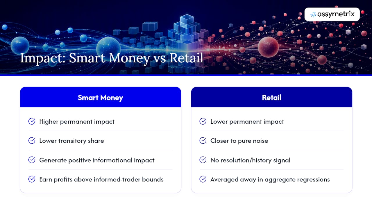
Research identifying price-sensitive traders in field prediction markets found that a subset of traders generate positive informational impact and earn profits above theoretical informed-trader lower bounds. Their trades push prices in a direction that tends to persist, which is the signature of genuine information rather than liquidity noise.
This is why a pure size-based impact model is incomplete. Orders of the same size in the same contract can produce different permanent-versus-transitory splits depending on the traders behind them. A GH regression run on aggregate flow averages this heterogeneity away, but a regression run on flow segmented by trader skill or wallet history recovers it.
Smart Money tracking exists precisely to address this gap. If you can flag wallets with a demonstrated edge, you can weight their flow more heavily in a permanent-impact estimate and treat unflagged retail flow as closer to pure noise. That segmentation turns a blunt Kyle lambda into something closer to a proper information-share model, and it’s the difference between an impact model that explains the past and one that anticipates the next repricing.
Thin markets amplify this effect further. With fewer participants absorbing flow, one informed wallet can move the price further and faster than the same wallet could in a deep, liquid contract, which is part of why whale detection matters more here than in equities.
Market Makers and Automated Liquidity on Price Dynamics
Market makers change the shape of the impact curve, not just its magnitude. A contract with active automated quoting on both sides absorbs moderate order flow with minimal price movement, then reprices sharply once flow exceeds the maker’s inventory tolerance. That produces a kinked, rather than smoothly concave, impact profile.

Automated liquidity provision in prediction markets tends to widen or pull quotes ahead of known resolution events, which is a rational response to adverse selection risk but a real problem for anyone trying to estimate a stable lambda. Depth measured on a quiet Tuesday can look nothing like depth measured the morning of a scheduled announcement, even in the same contract.
This matters directly for participation-rate decisions. A schedule calibrated against yesterday’s depth curve can badly misestimate slippage today if a market maker has stepped back. Practical models should treat depth as time-varying and refresh their estimate close to execution time, not rely on a static snapshot pulled hours earlier.
Maker behavior also interacts with the permanent-versus-temporary split. When makers actively provide two-sided quotes, more of an incoming order’s impact tends to look transitory, because the maker absorbs and later unwinds inventory rather than the price permanently repricing to new information. When makers withdraw, a comparable order looks far more permanent, simply because there’s no one left to absorb the temporary component. Tracking maker presence, inferred from quote density and quote-to-trade ratios in the orderbook feed, gives you a leading indicator of which regime you’re likely trading into.
How Event Uncertainty and Resolution Shape Impact
Impact behavior is not stationary across a contract’s life. Uncertainty about resolution timing and criteria widens the range of reasonable prices, which in practice means the depth curve is shallower and lambda is higher earlier in a contract’s life, then compresses again as resolution approaches and outcomes narrow.
Near resolution, two competing forces collide. Liquidity often collapses as market makers reduce exposure to binary settlement risk, which mechanically increases apparent impact per unit size. At the same time, genuinely informed traders with late information have their strongest incentive to trade right before resolution, since that’s when new information carries the most value relative to the time left to profit from it.
The calibration research across 292 million trades found calibration accuracy itself varies by horizon, meaning the raw price-to-probability mapping degrades unevenly as expiry nears. A price impact prediction markets model that uses a fixed lambda across the whole contract life will misestimate slippage badly in the final days, usually in the direction of overestimating available liquidity.
Ambiguous resolution criteria compound the problem. Contracts with disputed or unclear settlement rules tend to show erratic, non-concave impact patterns right before resolution, since traders are pricing settlement risk on top of outcome risk. Any production model should flag these contracts separately rather than pooling them with clean, well-defined markets in a single regression.
Statistical and Machine Learning Models for Binary Market Impact
Linear Kyle-style and GH regressions remain the right starting point because their coefficients are interpretable, but they assume a fixed relationship between flow and price that rarely holds across a contract’s entire life. Several extensions handle that better.
Quantile regression on log-odds returns captures how impact varies not just on average but at the tails, which matters given how much political and event contracts are driven by occasional large, informed trades rather than steady flow. Gradient-boosted trees and random forests can model the genuinely nonlinear, concave relationship between order size and impact without forcing a square-root functional form onto the data, at the cost of losing clean coefficient interpretation.
Sequence models, particularly ones that take recent trade sequences and orderbook snapshots as input, can pick up short-term momentum and mean-reversion patterns that a single-bin regression misses entirely. These work best layered on top of, not instead of, the GH and Kyle baselines, since the baselines still provide the interpretable permanent-versus-transitory decomposition that a black-box model can’t easily give you.
Whichever approach you choose, the square-root impact literature is a useful sanity check: if your fitted model implies impact that scales linearly or worse with size at typical trade sizes, something in the feature engineering or bin construction is likely off. Concavity should show up naturally in the data, not need to be forced by assumption.
Centralized vs Decentralized Prediction Markets and Impact
Kalshi operates as a centralized, regulated exchange with a traditional matching engine, while Polymarket settles trades on-chain against liquidity pools and orderbooks that interact with blockchain confirmation times. That structural difference shows up directly in impact measurement.
On-chain settlement introduces a latency layer that off-chain matching doesn’t have. A large order on a blockchain-based venue can experience impact from both the immediate orderbook response and from slippage introduced by transaction ordering and gas-price dynamics during confirmation. Centralized venues avoid that second layer entirely, since matching and settlement happen in the same system with no separate confirmation step.
Wallet-level transparency cuts the other way. On-chain venues expose full trade history tied to a wallet address, which makes the kind of informed-trader identification discussed earlier easier to build directly from public data. Centralized platforms typically require the venue’s own cooperation or a data partner to get comparable trader-level granularity.
Neither structure eliminates thin-book vulnerability. A whale can move price sharply on either type of venue when depth is shallow, but the mechanics of how that impact resolves, instant on a centralized matching engine, potentially delayed and gas-sensitive on-chain, mean a single impact model rarely transfers cleanly across venue types without recalibration.
A note on cross-platform generalization
A lambda estimated on Kalshi data will not transfer cleanly to Polymarket without recalibration. Platform-specific microstructure, fee structure, and settlement mechanics change the scale.
Wallet-level identification remains the most underused tool for separating informed traders from noise. It deserves more attention than aggregate flow models typically give it. The field would benefit from more open, pre-registered event-time replications rather than one-off case studies.
— Dean
Get the Orderbook and Trade Data to Build These Models Yourself
Assymetrix gives you normalized orderbook and trade feeds across Polymarket, Kalshi, and Limitless in one schema, so you never have to write three separate parsers before you can even start a lambda regression.
The Data API’s /sdk/markets/:id/orderbook and /sdk/markets/:id/trades endpoints return the price, size, side, and timestamp granularity this article’s models require, backed by roughly 1.5 terabytes of historical coverage for bootstrapping and event-time replication. If you’re building a production pipeline rather than a one-off study, the backtesting guide using Assymetrix historical snapshots walks through pulling trade-level data at scale and running it against a strategy. Start with the Data API developer guide to pull a sample orderbook snapshot and confirm the schema fits your existing regression pipeline before committing to a full historical backfill.
Sources
Decomposing crowd wisdom: domain-specific calibration dynamics in prediction markets
Price-sensitive traders and informational impact in field prediction markets
FAQ
Can You Actually Make Money Trading on Prediction Markets?
Some traders do, particularly those who identify informed order flow or exploit cross-venue mispricing, but research on price-sensitive traders found that a subset earn profits above theoretical informed-trader bounds. Most flow is closer to noise than edge.
How Often Do Large Price Corrections Happen in Binary Markets?
Sharp repricing tends to cluster around discrete resolution-relevant events rather than occurring on a fixed schedule. The 2024 election study found an assassination attempt produced far more permanent repricing than a scheduled debate, showing timing depends on information content, not calendar frequency.
Are Prediction Markets Actually Good at Forecasting Outcomes?
Accuracy varies by domain and time-to-expiry rather than being uniform. Calibration research across 292 million trades found persistent underconfidence in political markets, with prices compressed toward 50% even close to resolution.
Does Order Size Affect Price the Same Way on Every Platform?
No. Trade-size scale effects differ by venue microstructure, and the same calibration research found large trades on Kalshi produced disproportionate compression compared to equivalent trades elsewhere. Lambda estimates need platform-specific recalibration.
What Data Do I Need to Build a Price Impact Model?
You need trade-level data with price, size, side, and timestamp, plus orderbook depth snapshots at multiple price levels. Assymetrix’s /sdk/markets/:id/orderbook and /sdk/markets/:id/trades endpoints provide both in a normalized schema across Polymarket, Kalshi, and Limitless.
How Order Size Moves Prices in Prediction Markets
Price impact in binary prediction markets is concave: a larger order shifts the probability price meaningfully, but not in proportion to its size. Doubling a trade rarely doubles the move. Separating the permanent component from the temporary one requires a Glosten–Harris style decomposition and a Kyle-style lambda estimated on log-odds returns, not raw price.
Before modeling anything, compute four inputs:
Signed trade size and direction (buy/sell relative to the contract)
Net order flow aggregated into fixed time bins
Orderbook depth at each price level around the current mid
Participation rate: your order size relative to average volume in the window
Raw mid-price is not a usable probability without correction. Calibration drift by time-to-expiry, plus the bounded [0,1] price range, means a naive plug-in overstates confidence near the edges. A 292 million trade analysis across 327,000 binary contracts found systematic underconfidence in political markets, with prices compressed toward 50% even as resolution approached.
Key Takeaways
Price impact in binary prediction markets is concave and must be decomposed into permanent and temporary components using log-odds regressions before it can inform sizing decisions.
Point | Details |
|---|---|
Impact is concave, not linear | Larger orders move price less than proportionally, which is why slicing into smaller child orders reduces average execution cost. |
Decompose before you size | Use GH regressions and a Kyle-style lambda on log-odds returns to separate permanent, informational moves from temporary liquidity pressure. |
Horizon changes the model | Liquidity and calibration both shift as expiry nears, so a fixed lambda across a contract’s life will misestimate slippage. |
Wallet-level data reveals informed flow | Segmenting flow by trader history recovers information asymmetry that aggregate regressions average away. |
Assymetrix supplies the raw feeds | The |
Table of Contents
Price Impact Prediction Markets: Permanent vs Temporary Decomposition
Why Prediction Markets Differ From Equities and FX
Measuring Impact From Orderbook and Trade-Level Feeds
Sizing and Scheduling Execution to Limit Slippage
Building Price Impact Models With the Assymetrix Data API
Information Asymmetry as a Driver of Price Impact
Market Makers and Automated Liquidity on Price Dynamics
How Event Uncertainty and Resolution Shape Impact
Statistical and Machine Learning Models for Binary Market Impact
Centralized vs Decentralized Prediction Markets and Impact
Get the Orderbook and Trade Data to Build These Models Yourself
Sources
Price Impact Prediction Markets: Permanent vs Temporary Decomposition
Working in log-odds space, defined as ln(p / (1-p)), turns a bounded [0,1] probability into an unbounded real number, which is the correct scale for linear regression. Price changes near 0.05 or 0.95 compress heavily in raw terms but behave linearly in log-odds, so any serious price impact prediction markets model should transform first and interpret second.
The Glosten–Harris decomposition splits observed price change into two regressors: the order flow level, Q_t, which captures the permanent, information-driven component, and its first difference, ΔQ_t, which captures transitory liquidity pressure that mean-reverts. A coefficient near zero on ΔQ_t after controlling for Q_t suggests the market absorbs pressure quickly, a coefficient that stays large suggests thin depth.
A Kyle-style lambda, estimated by regressing log-odds changes on net signed order flow within fixed bins, gives you an effective-depth number directly comparable across markets and days.
Bin trades into 1 to 5 minute windows depending on venue activity.
Regress Δ log-odds on net signed flow to get lambda.
Compare lambda across contracts to rank liquidity depth.
Flag periods where gross flow is high but net flow is near zero.
That last step matters more in political contracts than in equities. Two-sided partisan flow can inflate lambda estimates if you only look at gross volume. An event-time study of the 2024 U.S. presidential contracts found the debate produced sharper transitory pressure, while the assassination attempt produced a more permanent repricing, evidence that the same dollar volume can carry very different information content depending on the shock.
Why Prediction Markets Differ From Equities and FX
A binary contract lives on [0, 1], and that bound changes the math. Impact near 0.5 looks nothing like impact near 0.05 or 0.95 in raw price terms, which is exactly why log-odds scaling exists. Near the extremes, a small absolute price move can represent a huge shift in relative confidence, and models that ignore this produce unstable, misleading lambda estimates.
Time-to-expiry adds a second distortion equities traders rarely worry about. Liquidity tends to collapse as resolution nears, and calibration itself drifts by horizon, a pattern the domain-specific calibration study documents directly. A market that looked deep well before expiry can turn thin fast.
Structural factors compound both effects:
Thin participation and pseudonymous wallets make it hard to distinguish informed flow from noise.
Partisan two-sided flow in political markets compresses prices toward the middle even when true probability sits at an extreme.
Trade-size scale effects vary by venue. The same $50,000 order can compress price differently on Kalshi than on Polymarket, purely due to microstructure differences in depth and order types.
Whale positioning in a thin book does more damage in prediction markets than in liquid FX pairs, simply because the counterparty pool is smaller and the resolution clock never stops ticking.
Measuring Impact From Orderbook and Trade-Level Feeds
Building a working price impact prediction markets model starts with picking the right dependent variable and matching it to the regressors that actually explain it. You have three reasonable targets: log-odds returns, raw mid-price moves, or immediate taker slippage against posted depth. Log-odds returns are the most stable choice for cross-market comparison.
Choose your dependent variable. Log-odds returns for cross-market work, taker slippage for execution-cost work.
Select regressors. Signed volume, net flow per bin, ΔQ_t (the transitory flow term), and participation rate relative to trailing average volume.
Run the Kyle-style template. Δ log-odds_t = λ · net_flow_t + controls, binned at 1 minute for active contracts and 5 minutes for thinner ones.
Run the GH regression alongside it. Regress log-odds change on both Q_t and ΔQ_t to separate the permanent estimate from the transitory one, then compare magnitudes.
Diagnose before trusting the output. Placebo tests on weekday-time windows with no news, bootstrapped confidence intervals across multiple days, a variance-ratio test to distinguish drift from reversal, and a two-sidedness index to catch offsetting partisan pressure.
Pro Tip: Run the two-sidedness index before you trust any lambda estimate from a political contract. Gross volume that’s mostly offsetting produces an artificially small apparent impact, hiding the true depth cost of a one-directional order.
Bin size | Best suited for | Tradeoff |
|---|---|---|
1 minute | High-volume contracts near major events | More noise, needs longer sample for stable lambda |
5 minutes | Moderate-activity markets | Smoother estimates, slower to catch fast-moving shocks |
Daily | Long-horizon calibration drift studies | Misses intraday impact entirely |
Theoretical work on metaorder impact and reaction-diffusion models supports concave, often square-root, scaling between order size and impact, which is the underlying reason slicing works at all in the next section.
Sizing and Scheduling Execution to Limit Slippage
Concave impact is the entire justification for slicing. If impact scales sub-linearly with size, breaking one large order into several smaller child orders reduces the average execution price compared to hitting the book once. TWAP and VWAP scheduling, along with participation-rate caps, exploit this directly, and analytic work on Hawkes-process impact models confirms that slicing improves average price under reasonable resilience assumptions.
Picking a participation rate depends on your lambda estimate. A market with a steep depth curve calls for a lower participation rate and a longer schedule; a deep, resilient market tolerates faster execution.
Estimate lambda and depth curve shape before setting a schedule, not after.
Cap participation rate as a percentage of trailing average volume, typically lower in thin contracts approaching expiry.
Run a short Monte Carlo across candidate schedules to compare expected slippage before committing capital.
Recheck depth intraday. Prediction market books move faster than equities books around news.
Pro Tip: Build your pre-trade checklist in this order: calibrate the probability input, estimate local depth from the current orderbook snapshot, then simulate two or three schedule options before choosing one. Skipping the calibration step is the most common source of bad sizing decisions.
Building Price Impact Models With the Assymetrix Data API
Two endpoints do most of the work: /sdk/markets/:id/orderbook for depth snapshots and /sdk/markets/:id/trades for trade-level flow. Extract price, size, side, timestamp, and wallet identifier where available from the trades endpoint, and pull depth at multiple price offsets from the orderbook endpoint so you can reconstruct the cost curve, not just the touch price.
Pull trades for the target market and window, filtering to the fields above.
Aggregate signed flow by wallet or by fixed time bin, matching your chosen bin size.
Convert mid-price to log-odds and compute returns.
Run the Kyle-style and GH regressions, then bootstrap confidence intervals across multiple days.
Cross-venue normalization is the part most quants underrate. Polymarket, Kalshi, and Limitless each structure their raw feeds differently, and pooling data across venues without a shared schema quietly poisons your regressions with scale mismatches. A normalized schema across venues removes that step from your pipeline entirely.
Roughly 1.5 terabytes of historical data spanning close to one billion rows of trading activity gives you enough event history to bootstrap confidence intervals properly and replicate event-time studies across dozens of comparable shocks, rather than relying on a single anecdotal case.
Wallet-level identification, covered in more depth in order flow analysis for prediction markets lets you separate informed flow from noise before you ever run the impact regression.
Event-Time Testing Checklist for Credible Results
Select markets with clean, timestamped events and confirm timestamp alignment to UTC.
Detect metaorders by clustering trades from the same wallet within short windows.
Test bin-size sensitivity by rerunning your regression at 1, 5, and 15 minute windows.
Adjust for exchange-specific fee structures before computing net returns.
Run weekday-time placebo windows, bootstrap confidence intervals, and check the two-sidedness index.
Watch for net-versus-gross flow confusion and platform-specific scale effects. Both distort lambda more than most researchers expect, particularly around large offsetting partisan orders.
Information Asymmetry as a Driver of Price Impact
Not all order flow carries the same information content, and that gap is what makes permanent impact possible in the first place. A trade from a wallet with a strong resolution record moves the price differently than an equal-sized trade from a wallet with no history, even though both hit the same depth curve.
Research identifying price-sensitive traders in field prediction markets found that a subset of traders generate positive informational impact and earn profits above theoretical informed-trader lower bounds. Their trades push prices in a direction that tends to persist, which is the signature of genuine information rather than liquidity noise.
This is why a pure size-based impact model is incomplete. Orders of the same size in the same contract can produce different permanent-versus-transitory splits depending on the traders behind them. A GH regression run on aggregate flow averages this heterogeneity away, but a regression run on flow segmented by trader skill or wallet history recovers it.
Smart Money tracking exists precisely to address this gap. If you can flag wallets with a demonstrated edge, you can weight their flow more heavily in a permanent-impact estimate and treat unflagged retail flow as closer to pure noise. That segmentation turns a blunt Kyle lambda into something closer to a proper information-share model, and it’s the difference between an impact model that explains the past and one that anticipates the next repricing.
Thin markets amplify this effect further. With fewer participants absorbing flow, one informed wallet can move the price further and faster than the same wallet could in a deep, liquid contract, which is part of why whale detection matters more here than in equities.
Market Makers and Automated Liquidity on Price Dynamics
Market makers change the shape of the impact curve, not just its magnitude. A contract with active automated quoting on both sides absorbs moderate order flow with minimal price movement, then reprices sharply once flow exceeds the maker’s inventory tolerance. That produces a kinked, rather than smoothly concave, impact profile.
Automated liquidity provision in prediction markets tends to widen or pull quotes ahead of known resolution events, which is a rational response to adverse selection risk but a real problem for anyone trying to estimate a stable lambda. Depth measured on a quiet Tuesday can look nothing like depth measured the morning of a scheduled announcement, even in the same contract.
This matters directly for participation-rate decisions. A schedule calibrated against yesterday’s depth curve can badly misestimate slippage today if a market maker has stepped back. Practical models should treat depth as time-varying and refresh their estimate close to execution time, not rely on a static snapshot pulled hours earlier.
Maker behavior also interacts with the permanent-versus-temporary split. When makers actively provide two-sided quotes, more of an incoming order’s impact tends to look transitory, because the maker absorbs and later unwinds inventory rather than the price permanently repricing to new information. When makers withdraw, a comparable order looks far more permanent, simply because there’s no one left to absorb the temporary component. Tracking maker presence, inferred from quote density and quote-to-trade ratios in the orderbook feed, gives you a leading indicator of which regime you’re likely trading into.
How Event Uncertainty and Resolution Shape Impact
Impact behavior is not stationary across a contract’s life. Uncertainty about resolution timing and criteria widens the range of reasonable prices, which in practice means the depth curve is shallower and lambda is higher earlier in a contract’s life, then compresses again as resolution approaches and outcomes narrow.
Near resolution, two competing forces collide. Liquidity often collapses as market makers reduce exposure to binary settlement risk, which mechanically increases apparent impact per unit size. At the same time, genuinely informed traders with late information have their strongest incentive to trade right before resolution, since that’s when new information carries the most value relative to the time left to profit from it.
The calibration research across 292 million trades found calibration accuracy itself varies by horizon, meaning the raw price-to-probability mapping degrades unevenly as expiry nears. A price impact prediction markets model that uses a fixed lambda across the whole contract life will misestimate slippage badly in the final days, usually in the direction of overestimating available liquidity.
Ambiguous resolution criteria compound the problem. Contracts with disputed or unclear settlement rules tend to show erratic, non-concave impact patterns right before resolution, since traders are pricing settlement risk on top of outcome risk. Any production model should flag these contracts separately rather than pooling them with clean, well-defined markets in a single regression.
Statistical and Machine Learning Models for Binary Market Impact
Linear Kyle-style and GH regressions remain the right starting point because their coefficients are interpretable, but they assume a fixed relationship between flow and price that rarely holds across a contract’s entire life. Several extensions handle that better.
Quantile regression on log-odds returns captures how impact varies not just on average but at the tails, which matters given how much political and event contracts are driven by occasional large, informed trades rather than steady flow. Gradient-boosted trees and random forests can model the genuinely nonlinear, concave relationship between order size and impact without forcing a square-root functional form onto the data, at the cost of losing clean coefficient interpretation.
Sequence models, particularly ones that take recent trade sequences and orderbook snapshots as input, can pick up short-term momentum and mean-reversion patterns that a single-bin regression misses entirely. These work best layered on top of, not instead of, the GH and Kyle baselines, since the baselines still provide the interpretable permanent-versus-transitory decomposition that a black-box model can’t easily give you.
Whichever approach you choose, the square-root impact literature is a useful sanity check: if your fitted model implies impact that scales linearly or worse with size at typical trade sizes, something in the feature engineering or bin construction is likely off. Concavity should show up naturally in the data, not need to be forced by assumption.
Centralized vs Decentralized Prediction Markets and Impact
Kalshi operates as a centralized, regulated exchange with a traditional matching engine, while Polymarket settles trades on-chain against liquidity pools and orderbooks that interact with blockchain confirmation times. That structural difference shows up directly in impact measurement.
On-chain settlement introduces a latency layer that off-chain matching doesn’t have. A large order on a blockchain-based venue can experience impact from both the immediate orderbook response and from slippage introduced by transaction ordering and gas-price dynamics during confirmation. Centralized venues avoid that second layer entirely, since matching and settlement happen in the same system with no separate confirmation step.
Wallet-level transparency cuts the other way. On-chain venues expose full trade history tied to a wallet address, which makes the kind of informed-trader identification discussed earlier easier to build directly from public data. Centralized platforms typically require the venue’s own cooperation or a data partner to get comparable trader-level granularity.
Neither structure eliminates thin-book vulnerability. A whale can move price sharply on either type of venue when depth is shallow, but the mechanics of how that impact resolves, instant on a centralized matching engine, potentially delayed and gas-sensitive on-chain, mean a single impact model rarely transfers cleanly across venue types without recalibration.
A note on cross-platform generalization
A lambda estimated on Kalshi data will not transfer cleanly to Polymarket without recalibration. Platform-specific microstructure, fee structure, and settlement mechanics change the scale.
Wallet-level identification remains the most underused tool for separating informed traders from noise. It deserves more attention than aggregate flow models typically give it. The field would benefit from more open, pre-registered event-time replications rather than one-off case studies.
— Dean
Get the Orderbook and Trade Data to Build These Models Yourself
Assymetrix gives you normalized orderbook and trade feeds across Polymarket, Kalshi, and Limitless in one schema, so you never have to write three separate parsers before you can even start a lambda regression.
The Data API’s /sdk/markets/:id/orderbook and /sdk/markets/:id/trades endpoints return the price, size, side, and timestamp granularity this article’s models require, backed by roughly 1.5 terabytes of historical coverage for bootstrapping and event-time replication. If you’re building a production pipeline rather than a one-off study, the backtesting guide using Assymetrix historical snapshots walks through pulling trade-level data at scale and running it against a strategy. Start with the Data API developer guide to pull a sample orderbook snapshot and confirm the schema fits your existing regression pipeline before committing to a full historical backfill.
Sources
Decomposing crowd wisdom: domain-specific calibration dynamics in prediction markets
Price-sensitive traders and informational impact in field prediction markets
FAQ
Can You Actually Make Money Trading on Prediction Markets?
Some traders do, particularly those who identify informed order flow or exploit cross-venue mispricing, but research on price-sensitive traders found that a subset earn profits above theoretical informed-trader bounds. Most flow is closer to noise than edge.
How Often Do Large Price Corrections Happen in Binary Markets?
Sharp repricing tends to cluster around discrete resolution-relevant events rather than occurring on a fixed schedule. The 2024 election study found an assassination attempt produced far more permanent repricing than a scheduled debate, showing timing depends on information content, not calendar frequency.
Are Prediction Markets Actually Good at Forecasting Outcomes?
Accuracy varies by domain and time-to-expiry rather than being uniform. Calibration research across 292 million trades found persistent underconfidence in political markets, with prices compressed toward 50% even close to resolution.
Does Order Size Affect Price the Same Way on Every Platform?
No. Trade-size scale effects differ by venue microstructure, and the same calibration research found large trades on Kalshi produced disproportionate compression compared to equivalent trades elsewhere. Lambda estimates need platform-specific recalibration.
What Data Do I Need to Build a Price Impact Model?
You need trade-level data with price, size, side, and timestamp, plus orderbook depth snapshots at multiple price levels. Assymetrix’s /sdk/markets/:id/orderbook and /sdk/markets/:id/trades endpoints provide both in a normalized schema across Polymarket, Kalshi, and Limitless.
Other Blog


