Prediction Market Liquidity: Unified API, Top 10 Depth, LAS for Devs
Prediction Market Liquidity: Unified API, Top 10 Depth, LAS for Devs
Prediction Market Liquidity: Unified API, Top 10 Depth, LAS for Devs
Developer and quant spec for prediction market liquidity: real time API with top 10 depth, precomputed LAS, and execution sizing rules.

Prediction Market Liquidity: Unified API, Top 10 Depth, LAS for Devs
The liquidity signals worth ingesting are quoted spread, effective spread (or Liquidity-Adjusted Spread), best-price and top-k order-book depth, short-horizon price impact, and daily volume paired with open interest. The immediate build step: pull L1 quotes, top-10 depth, and the trade stream, then compute effective spread and price impact at multiple sampling frequencies. A unified feed like the Assymetrix Data API handles cross-venue normalization; Polymarket-specific resources live at data.assymetrix.com/polymarket.
TL;DR:
Effective spread and top-k depth are critical for accurately measuring how much capital can move the market without adverse price impact, especially beyond the top of the book.
Most liquidity actually resides several levels back in the order book, so relying solely on top-of-book depth overstates tradable size and understates slippage risks.
Normalizing metrics across venues requires adjusting for fees, reconciling timestamps, and mapping markets to canonical IDs to enable meaningful cross-venue comparisons.
Liquidity should be monitored at multiple sampling frequencies and combined with impact-regression models for robust execution cost estimation and better trade sizing decisions.
Implementing liquidity-aware rules involves setting depth thresholds, capping trade sizes relative to visible depth, and dynamically adjusting order strategies based on real-time LAS and slippage estimates.
Assymetrixassymetrix.comBuild With Unified Liquidity DataAccess cross venue prediction market data through one integration, with order book coverage for developers, traders, and AI agents.Explore the Data API
Table of Contents
Prediction Market Liquidity Metrics: Definitions and Formulas
Reading Order-Book Depth and Shape Across Levels
Effective Spread, LAS, and What a Trade Really Costs
Measuring Price Impact and Adverse Selection
Volume, Open Interest, and When to Trust the Numbers
Turning Liquidity Metrics Into Trading Rules
What Institutional Liquidity Actually Changes
What a Liquidity API Should Actually Deliver
Making Liquidity Metrics Comparable Across Venues
Lessons From Building Liquidity-Aware Systems
Get Unified Liquidity Data Without Stitching Three Feeds Together
Sources
Prediction Market Liquidity Metrics: Definitions and Formulas
Liquidity in a prediction market is the capital available to move outcome shares without dragging the price against you. That single-sentence definition from Chainlink’s liquidity explainer is the right starting point, but it says nothing about how to compute the number your risk system actually needs. Below are the core formulas, written the way you’d implement them in a streaming pipeline.
Quoted spread is the gap between best bid and best ask: spread_q = ask_1 - bid_1. Mid-price is (bid_1 + ask_1) / 2. Both are trivial to compute but only describe the top of the book at a single instant, which is why they undersell true execution cost.
Effective spread corrects for that by using the actual trade price against the prevailing mid: spread_eff = 2 * |trade_price - mid_at_trade| . This captures cases where an order walks through several book levels, something the quoted spread never reflects.
Best-price depth is the size resting at bid_1 and ask_1. Cumulative top-k depth sums size across the first k levels on each side: depth_k = Σ(size_i) for i = 1 to k. Realized slippage measures the gap between the price you expected (the mid or the best quote at order submission) and your volume-weighted average fill price.
Sampling method changes what these numbers mean. Quote-frequency sampling captures every book update, which is noisy but complete. Trade-time sampling only records observations tied to executions, which biases toward active hours. Calendar-time sampling (every 1, 5, or 15 minutes) smooths for backtesting but can miss microstructure detail around news events. The Chainlink explainer’s recommendation to sample at multiple frequencies exists because book shape near contract resolution looks nothing like book shape mid-cycle. Run at least two of the three in parallel.
To compute these metrics consistently, your payload needs:
Timestamped best bid and ask, with sizes at each level
Full trade messages: price, size, and timestamp
Aggressor flag when the venue provides it (many public feeds don’t)
Top-k depth snapshots, not just L1
A canonical market ID that survives across sessions
Metric | Formula | Data required |
|---|---|---|
Quoted spread | ask_1 - bid_1 | L1 bid/ask |
Effective spread | 2 × | trade_price − mid |
Best-price depth | size at bid_1 / ask_1 | L1 sizes |
Cumulative top-k depth | Σ size_i, i=1…k | L1–Lk sizes |
Realized slippage | fill_avg_price − expected_price | trade fills, pre-trade mid |
Without the aggressor flag, effective spread still works because it only needs trade price and mid, not trade direction, as explained in the StockPilot Investor Insights Blog | AI Portfolio Strategy. Price impact regressions are where the missing sign field becomes a real problem, which the next section addresses directly.
Reading Order-Book Depth and Shape Across Levels
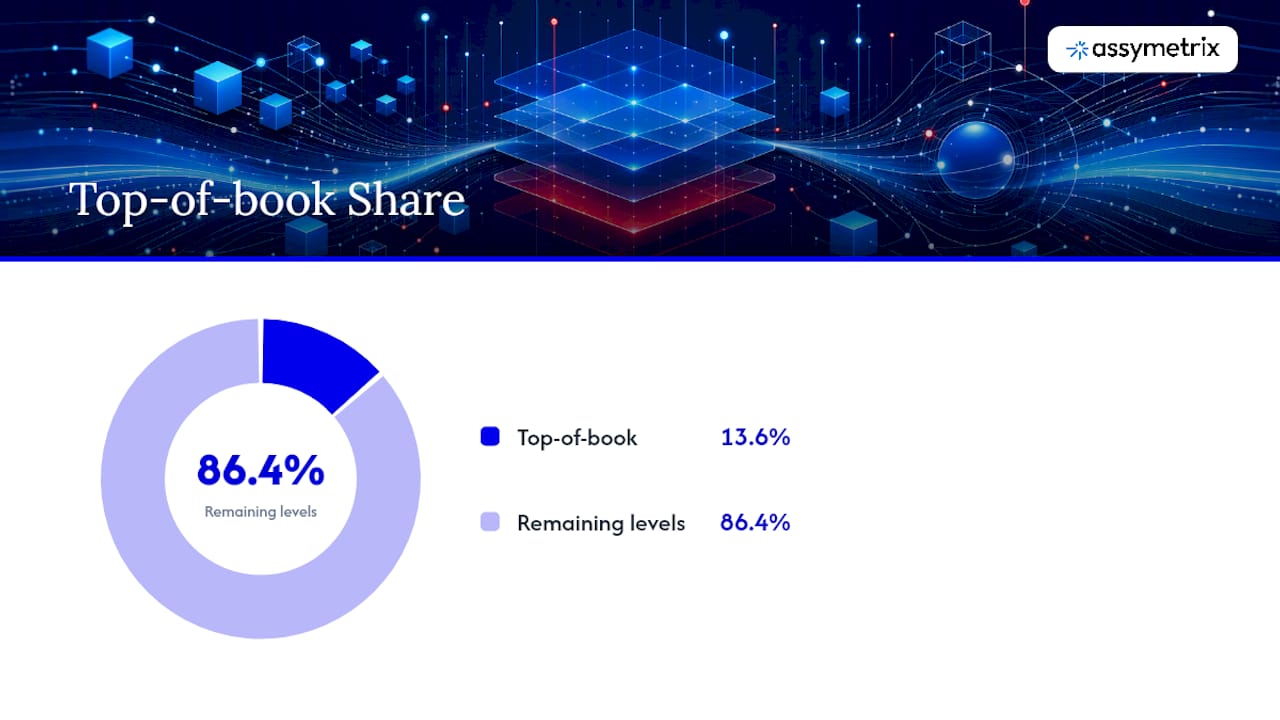
Depth at the top of the book tells you almost nothing about how a real order will fill. Research on Polymarket’s order book found the median top-of-book share sits around 0.136, meaning the best bid or ask typically holds only about 13.6% of the depth visible across the book. Most of the liquidity a large order actually eats sits several levels back, which is exactly why L1-only depth tracking underestimates fill risk for anything beyond a small clip.
Per-level depth is size_i at level i on either side. Cumulative depth at level k is the running sum from level 1 through k. Top-of-book share is size_1 / Σ(size_1...size_k), and a low share (below roughly 0.15, per the Polymarket finding) signals a layered book where you need to model multiple levels, not just the touch price.
Statistic to watch: median top-of-book share near 13.6% means naive L1-only liquidity checks systematically overstate how thin a book actually is, and understate how much size you can move before hitting real slippage.
A compact shape statistic worth computing alongside raw depth is a concentration measure, either a Herfindahl-style index across levels or a KL divergence between the observed depth distribution and a uniform reference. Either flags books that look deep in aggregate but are lopsided, with most size sitting on one side only.
A practical top-k depth payload for a 10-level book looks like:
bid_depth: [L1_size, L2_size, ..., L10_size]ask_depth: [L1_size, L2_size, ..., L10_size]timestamp,mid,concentration_index
For aggregation, use time-weighted averages over your sampling window rather than simple snapshots, and favor median windows over means since depth distributions are heavily right-skewed around news events. Sampling strictly on trade events biases your depth estimate toward moments right before or after fills, when the book is often temporarily thinner than its steady state. Sample on a fixed clock and reconcile against trade-time separately.
Effective Spread, LAS, and What a Trade Really Costs
Quoted spread tells you what the book looks like. It does not tell you what you’ll pay. That gap is why Market Math’s walkthrough of depth, spread, and slippage treats round-trip cost, not quoted spread, as the number that determines whether a signal survives execution.
Round-trip cost combines three components:
Effective spread on entry and exit, from actual fill prices against the mid at each trade
Platform fees, charged per trade or on the spread depending on venue
Slippage from depth consumption, when your order size exceeds what’s resting at the best price
Liquidity-Adjusted Spread (LAS) folds all three into a single post-cost number: LAS = effective_spread + fees + depth_slippage. Where the underlying reasoning behind standardizing a metric like this is straightforward: a raw probability edge of 3 cents means nothing if LAS eats 2.5 of those cents before you’re even flat.
Worked example: you spot a market priced at $0.42 where your model says fair value is $0.47, a 5 cent edge. The book shows a 1 cent quoted spread, but your order size of 5,000 shares needs to walk through three levels, producing a volume-weighted fill of $0.435. Your LAS comes out near 2.3 cents, cutting your theoretical edge by nearly half before you’ve even considered exit costs on the other side of the trade.
Component | Value |
|---|---|
Model edge | 5 cents |
Effective spread (fill vs. mid) | 1.5 cents |
Platform fee | 0.4 cents |
Depth slippage | 0.4 cents |
LAS (total drag) | 2.3¢ |
Net edge after LAS | 2.3 cents |
For sizing, feed LAS into your expected-value calculation before it ever reaches a Kelly formula. Run LAS as a pre-trade filter, not a post-trade reconciliation step.
Measuring Price Impact and Adverse Selection
Price impact tells you how much your own order moves the market, which matters more as your size grows relative to available depth. The standard estimator is a Kyle’s lambda style regression: Δmid = λ * signed_volume + ε, where λ is the price-impact coefficient you solve for via linear regression on historical trade and mid data. A higher λ means the same order size produces a bigger price move, a direct signal of thinner effective liquidity.
Realized short-horizon impact is simpler to compute directly: take the mid-price a fixed number of seconds after a trade and compare it to the pre-trade mid. This captures both the mechanical impact of consuming depth and any information content in the trade itself.
The complication: most public prediction market feeds don’t reliably flag which side was the aggressor. Microstructure research on Polymarket’s order book found that reconstructing aggressor sign from public data alone introduces meaningful noise, since trades near the mid can be misclassified in either direction.
Use midpoint sign heuristics (Lee-Ready style) as a fallback, comparing trade price to the prevailing mid
Cross-check against latency-aware timestamp alignment, since a trade logged slightly late can appear to fall on the wrong side of a mid-update
When sign confidence is low, fall back to unsigned impact measures rather than forcing a directional call
Track pass-through separately for large versus small trade proxies, since slow takers often absorb more adverse selection than fast ones
Pro Tip: Build your impact regression on unsigned volume first, then layer in sign inference as a confidence-weighted overlay. A model that only works with perfect aggressor flags breaks the moment you point it at a feed that doesn’t provide one.
Volume, Open Interest, and When to Trust the Numbers
Daily volume and open interest answer two different questions. Volume tells you how much capital changed hands today, a proxy for informed activity and short-term tradeability. Open interest tells you how much capital is currently committed to a market’s outcome, a proxy for how seriously the market is being priced.
Both metrics behave differently depending on when you sample them. Event-time sampling, meaning observations anchored to a specific occurrence like an earnings release or a debate, shows liquidity spiking sharply around the event and thinning fast afterward. Calendar-time sampling on the same market can miss that spike entirely if your window doesn’t align with it. Near contract resolution, spreads often tighten as certainty increases, then depth can evaporate suddenly once one outcome becomes near-certain and market makers pull quotes rather than hold inventory into a binary settlement.
Practical thresholds worth coding into an algo:
Require top-5 cumulative depth to be at least 3 to 5 times your intended order size before treating a market as tradeable at market price
Flag markets with daily volume below a rolling median as low-informed-activity, meaning quotes are more likely stale
Treat open interest that hasn’t moved in several sessions as a signal the market has gone dormant, regardless of what the spread looks like
Recompute all thresholds separately for near-resolution windows, since normal-regime depth rules don’t hold once a market is days from settling
Volume without depth context is a vanity metric. A market can show high daily volume from a handful of large trades against a thin book, which looks liquid on a headline chart but fails a real depth check the moment you try to size into it.
Turning Liquidity Metrics Into Trading Rules
Metrics only matter once they change what your algo actually does. The translation from measurement to decision rule is where most liquidity-aware systems either earn their edge or quietly bleed it away on bad fills.
Set a minimum depth threshold before choosing order type. If top-5 depth covers your full order size at an acceptable LAS, use a market order. If not, default to a limit order and let the book come to you.
Cap your share of visible depth. A common rule of thumb: never target more than 20 to 25% of top-5 cumulative depth in a single clip, splitting larger orders across time or price levels instead.
Use adaptive submission for size. Break large orders into smaller child orders, pausing or slowing submission around known event-time volatility windows rather than dumping size into a thin book.
Define an abort threshold. If realized slippage on the first slice of an order exceeds your pre-trade LAS estimate by a set margin, stop and reassess rather than continuing to execute into a book that’s moving against you.
Backtest against simulated fills, not quoted prices. Assuming every backtest fill happens at the quoted mid is the single most common way strategies look profitable on paper and lose money live.
Pro Tip: Run your backtest twice: once assuming naive fills at the quoted price, once simulating fills through actual top-k depth. The spread between those two backtest results is a rough estimate of how much of your paper edge is really execution cost in disguise. Assymetrix’s guide to estimating slippage from order-book depth walks through how to build that second simulation.
What Institutional Liquidity Actually Changes
Academic evidence on institutional participation in prediction markets gives a clearer picture than intuition alone. A synthetic microstructure study modeling market-maker coverage, liquidity incentives, and automation intensity found that moving from a low-institutional to a high-institutional liquidity regime compressed quoted spreads by roughly 14.1%, cut effective spreads by about 19.3%, increased depth by around 32.0%, and reduced short-horizon price impact by roughly 8.9%.
Those improvements did not distribute evenly. The same study found benefits pass through unevenly across trader types, and can actually worsen execution for slow takers during shock states, when fast institutional participants pull back first and leave slower orders exposed to a thinner book at the worst possible moment.
For measurement design, that unevenness is the actionable part. Don’t just track average spread and depth improvements; estimate pass-through separately by trader proxy (fast versus slow order submission patterns), and keep execution-quality metrics like effective spread and depth strictly separate from calibration metrics like Brier score or expected calibration error. A market can have excellent forecasting calibration and terrible execution quality at the same time, and conflating the two hides which problem you’re actually solving.
Sample spread and depth at multiple frequencies to catch regime shifts around shocks
Track pass-through by trader-speed proxy, not just in aggregate
Keep calibration metrics (Brier, ECE) reported separately from execution metrics (spread, depth, impact)
What a Liquidity API Should Actually Deliver
A real-time feed needs to expose more than a headline price. At minimum: bid, ask, mid, a timestamp with millisecond precision, a top-k depth vector (not just L1), and trade messages carrying price, size, and an aggressor flag where the venue supports it. Snapshot cadence should be configurable, since a market maker’s needs differ from a slower signal-generation pipeline running on 5-minute bars.
Batch and historical needs look different. You want a normalized trade ledger across sessions, canonical market IDs that survive relistings and don’t drift across venues, precomputed LAS and impact summaries so you’re not recomputing the same regression on every backtest run, and export formats that plug into standard research tooling (Parquet, CSV, or a Python-native interface).
Real-time: bid/ask/mid, timestamp, top-k depth vector, trade stream with aggressor flag when available
Batch: normalized trade ledger, canonical IDs, precomputed LAS, price-impact summaries, bulk export
Operational: clock synchronization across venues, documented rate limits, defined error handling, and canonicalization rules that keep the same underlying market mapped to one ID no matter which venue lists it
Requirement | Real-time need | Batch/historical need |
|---|---|---|
Depth | Top-k vector, sub-second | Full snapshot history |
Trades | Streamed with timestamp | Normalized ledger |
IDs | Canonical, cross-venue | Same, backward-compatible |
Derived metrics | Computed on ingest | Precomputed LAS, impact |
Time alignment is the detail that breaks the most pipelines. If your trade timestamps and your quote timestamps come from different clocks, even a few hundred milliseconds of drift can flip your aggressor-sign inference or misattribute a price move to the wrong trade. Assymetrix’s order-book integration guide covers the canonicalization rules needed to keep cross-venue timestamps aligned.
Making Liquidity Metrics Comparable Across Venues
Polymarket, Kalshi, and Limitless don’t charge fees the same way, don’t structure their order books identically, and don’t use the same market IDs for equivalent contracts. Comparing raw quoted spread across venues without adjusting for fees will make a cheaper-looking venue seem more liquid when it’s actually just charging costs differently.
The normalization workflow has four steps: map each venue’s market to a canonical ID representing the same underlying event, align timestamps to a common clock, convert quoted and effective spread into fee-adjusted LAS so the comparison reflects real cost, and compute depth-adjusted arbitrage feasibility, meaning whether the size available on both sides of a divergence actually supports the trade at a profitable net spread.
Canonicalize markets first; comparing spreads on differently mapped contracts produces meaningless deltas
Adjust every spread figure for venue-specific fees before ranking venues by cost
Compute depth-adjusted feasibility, not just price divergence, before flagging an arbitrage signal
Set divergence alert thresholds relative to combined LAS across both venues, not a flat cent value
Choose a venue-of-record for canonical pricing when multiple venues list overlapping markets, based on which shows deeper, more stable depth
Assymetrix’s guide to cross-venue arbitrage signals covers the divergence-threshold logic in more detail, including how depth-adjusted feasibility checks filter out signals that look profitable on price alone but fail once real execution cost enters the picture.
Lessons From Building Liquidity-Aware Systems
The biggest mistake teams make is trusting L1 depth as a proxy for tradeable size. It isn’t, and the Polymarket top-of-book data proves it: most of the book sits below the touch. The second mistake is treating aggressor sign as reliable when it’s inferred, not reported. Build your impact and pass-through models to degrade gracefully when that signal is noisy.
A working checklist: ingest L1 quotes plus top-10 depth plus the full trade stream, compute effective spread and LAS on every trade, simulate slippage through actual depth before trusting a backtest, and monitor pass-through by trader-speed proxy rather than assuming uniform execution quality. Iterate weekly, not quarterly. Assymetrix’s Python client guide is a reasonable place to see these pieces wired together in working code.
— Dean
Get Unified Liquidity Data Without Stitching Three Feeds Together
Building the pipeline described above means normalizing three venues that each structure depth, fees, and market IDs differently, then keeping that normalization correct as markets list, relist, and resolve. The Assymetrix Data API does that normalization once, so quoted spread, effective spread, top-k depth vectors, trade streams, and precomputed LAS and price-impact summaries arrive in a single schema across Polymarket, Kalshi, and Limitless.
The API ships canonical IDs that survive relistings, historical order-book archives for backtesting, and a real-time stream for live sizing decisions, all through one integration instead of three separate venue connections. Polymarket-specific documentation and sample payloads live at data.assymetrix.com/polymarket for teams starting there first. Start at data.assymetrix.com/api to pull a sample payload and test the top-k depth vectors against your own slippage model before committing to a full integration.
Sources
FAQ
How Do Prediction Markets Get Liquidity?
Liquidity comes from market makers posting quotes on both sides of the book, from traders placing limit orders that rest as depth, and increasingly from institutional participants running automated quoting strategies. Research on institutional liquidity channels shows that maker coverage and automation intensity together can meaningfully compress spreads and increase depth compared to markets with only retail participation.
What Is the Best Indicator for Liquidity?
No single indicator captures liquidity fully; effective spread and top-k cumulative depth together give the most complete picture because they reflect both cost and available size. Quoted spread alone understates true execution cost, which is why Liquidity-Adjusted Spread (LAS) is the more reliable metric for expected-value calculations.
How Do You Measure Market Liquidity?
Market liquidity is measured through a combination of spread, depth, and slippage: quoted and effective spread capture cost, top-k depth capture available size, and realized slippage captures the gap between expected and actual fill price. Simulating execution through actual depth levels, rather than assuming fills at the quoted price, produces the most accurate liquidity estimate.
What Do Liquidity Metrics Measure?
Liquidity metrics measure how much capital a market can absorb before prices move meaningfully, covering three dimensions: cost to trade (spread), available size (depth), and the price impact of your own order. Assymetrix’s Data API delivers all three, normalized across venues, so teams don’t have to reconstruct these calculations separately for Polymarket, Kalshi, and Limitless.
Why Does Liquidity Vary So Much Between Prediction Market Venues?
Liquidity differs across venues because of different fee structures, different maker incentive programs, and different participant mixes, ranging from mostly retail order flow to heavier institutional and automated market-making presence. Comparing raw spread or depth numbers across venues without adjusting for these differences produces misleading rankings, which is why fee-adjusted, canonicalized comparisons matter for any cross-venue signal.
Prediction Market Liquidity: Unified API, Top 10 Depth, LAS for Devs
The liquidity signals worth ingesting are quoted spread, effective spread (or Liquidity-Adjusted Spread), best-price and top-k order-book depth, short-horizon price impact, and daily volume paired with open interest. The immediate build step: pull L1 quotes, top-10 depth, and the trade stream, then compute effective spread and price impact at multiple sampling frequencies. A unified feed like the Assymetrix Data API handles cross-venue normalization; Polymarket-specific resources live at data.assymetrix.com/polymarket.
TL;DR:
Effective spread and top-k depth are critical for accurately measuring how much capital can move the market without adverse price impact, especially beyond the top of the book.
Most liquidity actually resides several levels back in the order book, so relying solely on top-of-book depth overstates tradable size and understates slippage risks.
Normalizing metrics across venues requires adjusting for fees, reconciling timestamps, and mapping markets to canonical IDs to enable meaningful cross-venue comparisons.
Liquidity should be monitored at multiple sampling frequencies and combined with impact-regression models for robust execution cost estimation and better trade sizing decisions.
Implementing liquidity-aware rules involves setting depth thresholds, capping trade sizes relative to visible depth, and dynamically adjusting order strategies based on real-time LAS and slippage estimates.
Assymetrixassymetrix.comBuild With Unified Liquidity DataAccess cross venue prediction market data through one integration, with order book coverage for developers, traders, and AI agents.Explore the Data API
Table of Contents
Prediction Market Liquidity Metrics: Definitions and Formulas
Reading Order-Book Depth and Shape Across Levels
Effective Spread, LAS, and What a Trade Really Costs
Measuring Price Impact and Adverse Selection
Volume, Open Interest, and When to Trust the Numbers
Turning Liquidity Metrics Into Trading Rules
What Institutional Liquidity Actually Changes
What a Liquidity API Should Actually Deliver
Making Liquidity Metrics Comparable Across Venues
Lessons From Building Liquidity-Aware Systems
Get Unified Liquidity Data Without Stitching Three Feeds Together
Sources
Prediction Market Liquidity Metrics: Definitions and Formulas
Liquidity in a prediction market is the capital available to move outcome shares without dragging the price against you. That single-sentence definition from Chainlink’s liquidity explainer is the right starting point, but it says nothing about how to compute the number your risk system actually needs. Below are the core formulas, written the way you’d implement them in a streaming pipeline.
Quoted spread is the gap between best bid and best ask: spread_q = ask_1 - bid_1. Mid-price is (bid_1 + ask_1) / 2. Both are trivial to compute but only describe the top of the book at a single instant, which is why they undersell true execution cost.
Effective spread corrects for that by using the actual trade price against the prevailing mid: spread_eff = 2 * |trade_price - mid_at_trade| . This captures cases where an order walks through several book levels, something the quoted spread never reflects.
Best-price depth is the size resting at bid_1 and ask_1. Cumulative top-k depth sums size across the first k levels on each side: depth_k = Σ(size_i) for i = 1 to k. Realized slippage measures the gap between the price you expected (the mid or the best quote at order submission) and your volume-weighted average fill price.
Sampling method changes what these numbers mean. Quote-frequency sampling captures every book update, which is noisy but complete. Trade-time sampling only records observations tied to executions, which biases toward active hours. Calendar-time sampling (every 1, 5, or 15 minutes) smooths for backtesting but can miss microstructure detail around news events. The Chainlink explainer’s recommendation to sample at multiple frequencies exists because book shape near contract resolution looks nothing like book shape mid-cycle. Run at least two of the three in parallel.
To compute these metrics consistently, your payload needs:
Timestamped best bid and ask, with sizes at each level
Full trade messages: price, size, and timestamp
Aggressor flag when the venue provides it (many public feeds don’t)
Top-k depth snapshots, not just L1
A canonical market ID that survives across sessions
Metric | Formula | Data required |
|---|---|---|
Quoted spread | ask_1 - bid_1 | L1 bid/ask |
Effective spread | 2 × | trade_price − mid |
Best-price depth | size at bid_1 / ask_1 | L1 sizes |
Cumulative top-k depth | Σ size_i, i=1…k | L1–Lk sizes |
Realized slippage | fill_avg_price − expected_price | trade fills, pre-trade mid |
Without the aggressor flag, effective spread still works because it only needs trade price and mid, not trade direction, as explained in the StockPilot Investor Insights Blog | AI Portfolio Strategy. Price impact regressions are where the missing sign field becomes a real problem, which the next section addresses directly.
Reading Order-Book Depth and Shape Across Levels
Depth at the top of the book tells you almost nothing about how a real order will fill. Research on Polymarket’s order book found the median top-of-book share sits around 0.136, meaning the best bid or ask typically holds only about 13.6% of the depth visible across the book. Most of the liquidity a large order actually eats sits several levels back, which is exactly why L1-only depth tracking underestimates fill risk for anything beyond a small clip.
Per-level depth is size_i at level i on either side. Cumulative depth at level k is the running sum from level 1 through k. Top-of-book share is size_1 / Σ(size_1...size_k), and a low share (below roughly 0.15, per the Polymarket finding) signals a layered book where you need to model multiple levels, not just the touch price.
Statistic to watch: median top-of-book share near 13.6% means naive L1-only liquidity checks systematically overstate how thin a book actually is, and understate how much size you can move before hitting real slippage.
A compact shape statistic worth computing alongside raw depth is a concentration measure, either a Herfindahl-style index across levels or a KL divergence between the observed depth distribution and a uniform reference. Either flags books that look deep in aggregate but are lopsided, with most size sitting on one side only.
A practical top-k depth payload for a 10-level book looks like:
bid_depth: [L1_size, L2_size, ..., L10_size]ask_depth: [L1_size, L2_size, ..., L10_size]timestamp,mid,concentration_index
For aggregation, use time-weighted averages over your sampling window rather than simple snapshots, and favor median windows over means since depth distributions are heavily right-skewed around news events. Sampling strictly on trade events biases your depth estimate toward moments right before or after fills, when the book is often temporarily thinner than its steady state. Sample on a fixed clock and reconcile against trade-time separately.
Effective Spread, LAS, and What a Trade Really Costs
Quoted spread tells you what the book looks like. It does not tell you what you’ll pay. That gap is why Market Math’s walkthrough of depth, spread, and slippage treats round-trip cost, not quoted spread, as the number that determines whether a signal survives execution.
Round-trip cost combines three components:
Effective spread on entry and exit, from actual fill prices against the mid at each trade
Platform fees, charged per trade or on the spread depending on venue
Slippage from depth consumption, when your order size exceeds what’s resting at the best price
Liquidity-Adjusted Spread (LAS) folds all three into a single post-cost number: LAS = effective_spread + fees + depth_slippage. Where the underlying reasoning behind standardizing a metric like this is straightforward: a raw probability edge of 3 cents means nothing if LAS eats 2.5 of those cents before you’re even flat.
Worked example: you spot a market priced at $0.42 where your model says fair value is $0.47, a 5 cent edge. The book shows a 1 cent quoted spread, but your order size of 5,000 shares needs to walk through three levels, producing a volume-weighted fill of $0.435. Your LAS comes out near 2.3 cents, cutting your theoretical edge by nearly half before you’ve even considered exit costs on the other side of the trade.
Component | Value |
|---|---|
Model edge | 5 cents |
Effective spread (fill vs. mid) | 1.5 cents |
Platform fee | 0.4 cents |
Depth slippage | 0.4 cents |
LAS (total drag) | 2.3¢ |
Net edge after LAS | 2.3 cents |
For sizing, feed LAS into your expected-value calculation before it ever reaches a Kelly formula. Run LAS as a pre-trade filter, not a post-trade reconciliation step.
Measuring Price Impact and Adverse Selection
Price impact tells you how much your own order moves the market, which matters more as your size grows relative to available depth. The standard estimator is a Kyle’s lambda style regression: Δmid = λ * signed_volume + ε, where λ is the price-impact coefficient you solve for via linear regression on historical trade and mid data. A higher λ means the same order size produces a bigger price move, a direct signal of thinner effective liquidity.
Realized short-horizon impact is simpler to compute directly: take the mid-price a fixed number of seconds after a trade and compare it to the pre-trade mid. This captures both the mechanical impact of consuming depth and any information content in the trade itself.
The complication: most public prediction market feeds don’t reliably flag which side was the aggressor. Microstructure research on Polymarket’s order book found that reconstructing aggressor sign from public data alone introduces meaningful noise, since trades near the mid can be misclassified in either direction.
Use midpoint sign heuristics (Lee-Ready style) as a fallback, comparing trade price to the prevailing mid
Cross-check against latency-aware timestamp alignment, since a trade logged slightly late can appear to fall on the wrong side of a mid-update
When sign confidence is low, fall back to unsigned impact measures rather than forcing a directional call
Track pass-through separately for large versus small trade proxies, since slow takers often absorb more adverse selection than fast ones
Pro Tip: Build your impact regression on unsigned volume first, then layer in sign inference as a confidence-weighted overlay. A model that only works with perfect aggressor flags breaks the moment you point it at a feed that doesn’t provide one.
Volume, Open Interest, and When to Trust the Numbers
Daily volume and open interest answer two different questions. Volume tells you how much capital changed hands today, a proxy for informed activity and short-term tradeability. Open interest tells you how much capital is currently committed to a market’s outcome, a proxy for how seriously the market is being priced.
Both metrics behave differently depending on when you sample them. Event-time sampling, meaning observations anchored to a specific occurrence like an earnings release or a debate, shows liquidity spiking sharply around the event and thinning fast afterward. Calendar-time sampling on the same market can miss that spike entirely if your window doesn’t align with it. Near contract resolution, spreads often tighten as certainty increases, then depth can evaporate suddenly once one outcome becomes near-certain and market makers pull quotes rather than hold inventory into a binary settlement.
Practical thresholds worth coding into an algo:
Require top-5 cumulative depth to be at least 3 to 5 times your intended order size before treating a market as tradeable at market price
Flag markets with daily volume below a rolling median as low-informed-activity, meaning quotes are more likely stale
Treat open interest that hasn’t moved in several sessions as a signal the market has gone dormant, regardless of what the spread looks like
Recompute all thresholds separately for near-resolution windows, since normal-regime depth rules don’t hold once a market is days from settling
Volume without depth context is a vanity metric. A market can show high daily volume from a handful of large trades against a thin book, which looks liquid on a headline chart but fails a real depth check the moment you try to size into it.
Turning Liquidity Metrics Into Trading Rules
Metrics only matter once they change what your algo actually does. The translation from measurement to decision rule is where most liquidity-aware systems either earn their edge or quietly bleed it away on bad fills.
Set a minimum depth threshold before choosing order type. If top-5 depth covers your full order size at an acceptable LAS, use a market order. If not, default to a limit order and let the book come to you.
Cap your share of visible depth. A common rule of thumb: never target more than 20 to 25% of top-5 cumulative depth in a single clip, splitting larger orders across time or price levels instead.
Use adaptive submission for size. Break large orders into smaller child orders, pausing or slowing submission around known event-time volatility windows rather than dumping size into a thin book.
Define an abort threshold. If realized slippage on the first slice of an order exceeds your pre-trade LAS estimate by a set margin, stop and reassess rather than continuing to execute into a book that’s moving against you.
Backtest against simulated fills, not quoted prices. Assuming every backtest fill happens at the quoted mid is the single most common way strategies look profitable on paper and lose money live.
Pro Tip: Run your backtest twice: once assuming naive fills at the quoted price, once simulating fills through actual top-k depth. The spread between those two backtest results is a rough estimate of how much of your paper edge is really execution cost in disguise. Assymetrix’s guide to estimating slippage from order-book depth walks through how to build that second simulation.
What Institutional Liquidity Actually Changes
Academic evidence on institutional participation in prediction markets gives a clearer picture than intuition alone. A synthetic microstructure study modeling market-maker coverage, liquidity incentives, and automation intensity found that moving from a low-institutional to a high-institutional liquidity regime compressed quoted spreads by roughly 14.1%, cut effective spreads by about 19.3%, increased depth by around 32.0%, and reduced short-horizon price impact by roughly 8.9%.
Those improvements did not distribute evenly. The same study found benefits pass through unevenly across trader types, and can actually worsen execution for slow takers during shock states, when fast institutional participants pull back first and leave slower orders exposed to a thinner book at the worst possible moment.
For measurement design, that unevenness is the actionable part. Don’t just track average spread and depth improvements; estimate pass-through separately by trader proxy (fast versus slow order submission patterns), and keep execution-quality metrics like effective spread and depth strictly separate from calibration metrics like Brier score or expected calibration error. A market can have excellent forecasting calibration and terrible execution quality at the same time, and conflating the two hides which problem you’re actually solving.
Sample spread and depth at multiple frequencies to catch regime shifts around shocks
Track pass-through by trader-speed proxy, not just in aggregate
Keep calibration metrics (Brier, ECE) reported separately from execution metrics (spread, depth, impact)
What a Liquidity API Should Actually Deliver
A real-time feed needs to expose more than a headline price. At minimum: bid, ask, mid, a timestamp with millisecond precision, a top-k depth vector (not just L1), and trade messages carrying price, size, and an aggressor flag where the venue supports it. Snapshot cadence should be configurable, since a market maker’s needs differ from a slower signal-generation pipeline running on 5-minute bars.
Batch and historical needs look different. You want a normalized trade ledger across sessions, canonical market IDs that survive relistings and don’t drift across venues, precomputed LAS and impact summaries so you’re not recomputing the same regression on every backtest run, and export formats that plug into standard research tooling (Parquet, CSV, or a Python-native interface).
Real-time: bid/ask/mid, timestamp, top-k depth vector, trade stream with aggressor flag when available
Batch: normalized trade ledger, canonical IDs, precomputed LAS, price-impact summaries, bulk export
Operational: clock synchronization across venues, documented rate limits, defined error handling, and canonicalization rules that keep the same underlying market mapped to one ID no matter which venue lists it
Requirement | Real-time need | Batch/historical need |
|---|---|---|
Depth | Top-k vector, sub-second | Full snapshot history |
Trades | Streamed with timestamp | Normalized ledger |
IDs | Canonical, cross-venue | Same, backward-compatible |
Derived metrics | Computed on ingest | Precomputed LAS, impact |
Time alignment is the detail that breaks the most pipelines. If your trade timestamps and your quote timestamps come from different clocks, even a few hundred milliseconds of drift can flip your aggressor-sign inference or misattribute a price move to the wrong trade. Assymetrix’s order-book integration guide covers the canonicalization rules needed to keep cross-venue timestamps aligned.
Making Liquidity Metrics Comparable Across Venues
Polymarket, Kalshi, and Limitless don’t charge fees the same way, don’t structure their order books identically, and don’t use the same market IDs for equivalent contracts. Comparing raw quoted spread across venues without adjusting for fees will make a cheaper-looking venue seem more liquid when it’s actually just charging costs differently.
The normalization workflow has four steps: map each venue’s market to a canonical ID representing the same underlying event, align timestamps to a common clock, convert quoted and effective spread into fee-adjusted LAS so the comparison reflects real cost, and compute depth-adjusted arbitrage feasibility, meaning whether the size available on both sides of a divergence actually supports the trade at a profitable net spread.
Canonicalize markets first; comparing spreads on differently mapped contracts produces meaningless deltas
Adjust every spread figure for venue-specific fees before ranking venues by cost
Compute depth-adjusted feasibility, not just price divergence, before flagging an arbitrage signal
Set divergence alert thresholds relative to combined LAS across both venues, not a flat cent value
Choose a venue-of-record for canonical pricing when multiple venues list overlapping markets, based on which shows deeper, more stable depth
Assymetrix’s guide to cross-venue arbitrage signals covers the divergence-threshold logic in more detail, including how depth-adjusted feasibility checks filter out signals that look profitable on price alone but fail once real execution cost enters the picture.
Lessons From Building Liquidity-Aware Systems
The biggest mistake teams make is trusting L1 depth as a proxy for tradeable size. It isn’t, and the Polymarket top-of-book data proves it: most of the book sits below the touch. The second mistake is treating aggressor sign as reliable when it’s inferred, not reported. Build your impact and pass-through models to degrade gracefully when that signal is noisy.
A working checklist: ingest L1 quotes plus top-10 depth plus the full trade stream, compute effective spread and LAS on every trade, simulate slippage through actual depth before trusting a backtest, and monitor pass-through by trader-speed proxy rather than assuming uniform execution quality. Iterate weekly, not quarterly. Assymetrix’s Python client guide is a reasonable place to see these pieces wired together in working code.
— Dean
Get Unified Liquidity Data Without Stitching Three Feeds Together
Building the pipeline described above means normalizing three venues that each structure depth, fees, and market IDs differently, then keeping that normalization correct as markets list, relist, and resolve. The Assymetrix Data API does that normalization once, so quoted spread, effective spread, top-k depth vectors, trade streams, and precomputed LAS and price-impact summaries arrive in a single schema across Polymarket, Kalshi, and Limitless.
The API ships canonical IDs that survive relistings, historical order-book archives for backtesting, and a real-time stream for live sizing decisions, all through one integration instead of three separate venue connections. Polymarket-specific documentation and sample payloads live at data.assymetrix.com/polymarket for teams starting there first. Start at data.assymetrix.com/api to pull a sample payload and test the top-k depth vectors against your own slippage model before committing to a full integration.
Sources
FAQ
How Do Prediction Markets Get Liquidity?
Liquidity comes from market makers posting quotes on both sides of the book, from traders placing limit orders that rest as depth, and increasingly from institutional participants running automated quoting strategies. Research on institutional liquidity channels shows that maker coverage and automation intensity together can meaningfully compress spreads and increase depth compared to markets with only retail participation.
What Is the Best Indicator for Liquidity?
No single indicator captures liquidity fully; effective spread and top-k cumulative depth together give the most complete picture because they reflect both cost and available size. Quoted spread alone understates true execution cost, which is why Liquidity-Adjusted Spread (LAS) is the more reliable metric for expected-value calculations.
How Do You Measure Market Liquidity?
Market liquidity is measured through a combination of spread, depth, and slippage: quoted and effective spread capture cost, top-k depth capture available size, and realized slippage captures the gap between expected and actual fill price. Simulating execution through actual depth levels, rather than assuming fills at the quoted price, produces the most accurate liquidity estimate.
What Do Liquidity Metrics Measure?
Liquidity metrics measure how much capital a market can absorb before prices move meaningfully, covering three dimensions: cost to trade (spread), available size (depth), and the price impact of your own order. Assymetrix’s Data API delivers all three, normalized across venues, so teams don’t have to reconstruct these calculations separately for Polymarket, Kalshi, and Limitless.
Why Does Liquidity Vary So Much Between Prediction Market Venues?
Liquidity differs across venues because of different fee structures, different maker incentive programs, and different participant mixes, ranging from mostly retail order flow to heavier institutional and automated market-making presence. Comparing raw spread or depth numbers across venues without adjusting for these differences produces misleading rankings, which is why fee-adjusted, canonicalized comparisons matter for any cross-venue signal.
Other Blog


