Parquet Prediction Market Data: Schema, Encoding, Queries

Parquet is the right default for prediction market history once you pass a few gigabytes: it is columnar, compressed, and readable by DuckDB, Spark, pandas and Polars without a database server. The format is the easy part. What decides whether your Parquet files are usable is the schema you write into them, how you encode timestamps, and which clock you trust. This guide covers all three, with the queries to prove it.

AssymetrixSkip the Prediction Data Collection WorkAssymetrix brings Polymarket, Kalshi, and Limitless data together through one API, with historical coverage for prediction market research.Explore the Data API

TL;DR

• Enforce one canonical schema at ingestion, before you write any Parquet, instead of merging venue schemas at read time.

• Partition by venue and date, keep timestamps as integers, and let dictionary encoding handle categorical columns such as outcome and side.

• Store the venue-ingest timestamp next to the event timestamp. Backtests that use the wrong one leak the future.

• Cross-venue price gaps often reflect different resolution rules, so your files need an event-identity column, not just a market title.

• Query with predicate pushdown (DuckDB or Arrow) and never load the full history into memory.

Table of Contents

• Why Parquet fits prediction market data

• Design the schema before you write a file

• Encoding and compression that pay off

• Partitioning: venue first, then date

• Querying it with DuckDB

• The clock problem: which timestamp can you trust?

• From files to a backtest

• Feeding AI agents from Parquet

• Our perspective on Parquet and prediction market data

• Skip the collection work

• FAQ

• Sources

Why Parquet fits prediction market data

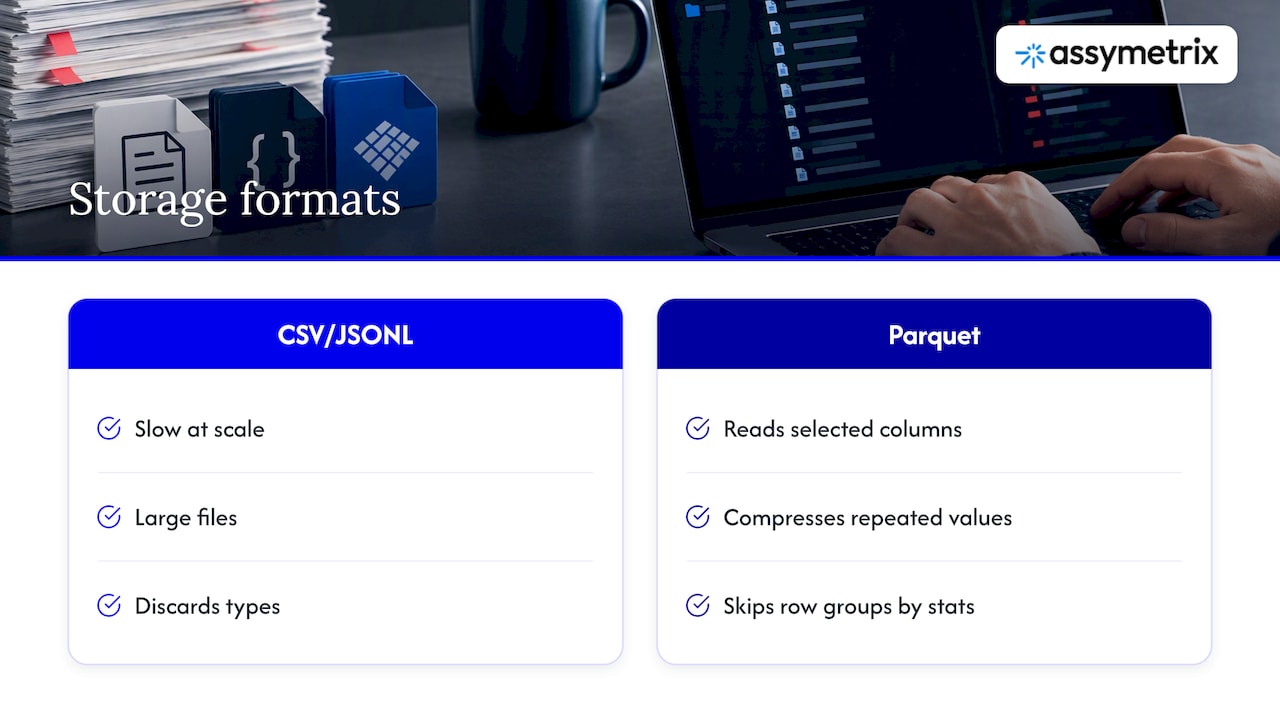
Prediction market data is tall and narrow. A trade or order book update is a handful of fields: a market identifier, an outcome, a price between 0 and 1, a size, a side, a timestamp. Multiply that by hundreds of millions of rows and a row-oriented format such as CSV or JSON lines becomes slow, large and lossy (it discards types).

Columnar storage changes the economics. Queries that touch only price and ts read only those columns. Repeated values such as venue names, outcome labels and sides compress to almost nothing. Parquet also stores min/max statistics per row group, so an engine can skip whole chunks of a file when you filter by time or market. Apache Parquet and Apache Arrow internals is a solid explainer of how Parquet suits durable storage while Arrow suits in-memory processing, and why the two are designed to work together.

The practical consequence: a quant on a laptop can run a month-long, three-venue backtest query in seconds, provided the files are laid out well. Most of this article is about that layout.

Design the schema before you write a file

The most expensive mistake is writing each venue’s native payload to its own Parquet files and planning to reconcile later. Polymarket, Kalshi and Limitless describe markets differently: different identifiers, different outcome conventions, different price units and tick sizes. If the files disagree, every downstream query pays for it.

DuckDB documents union_by_name for loading Parquet files with different schemas. It works, but treat it as a rescue tool. Enforcing the unified schema at the ingestion layer, in the database or pipeline stage that precedes the Parquet export, is cheaper than reconciling at read time on every query, and it keeps types consistent across years of files.

A minimal canonical trade table looks like this:

Two columns deserve special attention: the canonical market ID and the dual timestamps.

Canonical IDs are an analytics feature, not a convenience

Researchers at TUM studying 100,000+ events found that semantically equivalent markets are rarely interchangeable: platform-specific resolution rules mean that two contracts about the same headline can settle differently. Their finding is that median price deviations sit roughly 2 to 4% away from parity, and that this is largely a structural limit on how platforms define event identity, not simply disagreement about information.

For your Parquet layout, that means a canonical_market_id alone is not enough for arbitrage research. Add a resolution_rule_hash or a free-text resolution_source column so you can later separate true duplicates from look-alikes. Otherwise a backtest will show a spread that no one could have closed.

If you would rather not build the mapping yourself, our cross-venue canonical ID guide explains how we normalize identifiers across venues.

Encoding and compression that pay off

For high-frequency order book or trade data, a few settings make most of the difference:

1. Timestamps as integers with delta encoding. Consecutive timestamps in a sorted file differ by small amounts, which is exactly what Parquet’s DELTA_BINARY_PACKED encoding exploits. Store epoch milliseconds or microseconds as int64 rather than strings or naive datetimes.

2. Dictionary encoding for categoricals. Columns such as venue, outcome and side have a handful of distinct values across millions of rows. Dictionary encoding shrinks them to a few bits per value.

3. ZSTD compression. A higher ZSTD level costs write time and pays back in storage and read bandwidth. For archives written once and read many times, that is a good trade. Test levels on one day of your own data before committing.

4. Sort before you write. Sort by canonical_market_id, then ts_event. Sorted data makes delta encoding tighter and row-group min/max statistics far more selective.

5. Moderate row groups. Row groups of roughly a million rows, or about 128 MB, are a common starting point. Smaller groups give finer skipping but more metadata. Measure on your queries.

Here is a pyarrow write that applies the above:

import pyarrow as pa
import pyarrow.parquet as pq

table = table.sort_by([("canonical_market_id", "ascending"),
                       ("ts_event", "ascending")])

pq.write_table(
    table,
    "trades/venue=kalshi/date=2026-10-19/part-000.parquet",
    compression="zstd",
    compression_level=9,
    use_dictionary=["venue", "outcome", "side"],
    column_encoding={"ts_event": "DELTA_BINARY_PACKED",
                     "ts_ingest": "DELTA_BINARY_PACKED"},
    row_group_size=1_000_000,
)

import pyarrow as pa
import pyarrow.parquet as pq

table = table.sort_by([("canonical_market_id", "ascending"),
                       ("ts_event", "ascending")])

pq.write_table(
    table,
    "trades/venue=kalshi/date=2026-10-19/part-000.parquet",
    compression="zstd",
    compression_level=9,
    use_dictionary=["venue", "outcome", "side"],
    column_encoding={"ts_event": "DELTA_BINARY_PACKED",
                     "ts_ingest": "DELTA_BINARY_PACKED"},
    row_group_size=1_000_000,
)

Note that pyarrow requires dictionary encoding to be disabled for any column you assign an explicit encoding, so pass use_dictionary as a list of the columns you want dictionary-encoded, as above.

Partitioning: venue first, then date

Partition layout is how engines avoid reading files at all. A Hive-style directory tree is the standard:

trades/
  venue=polymarket/date=2026-10-19/part-000.parquet
  venue=kalshi/date=2026-10-19/part-000.parquet
  venue=limitless/date=2026-10-19/part-000.parquet

trades/
  venue=polymarket/date=2026-10-19/part-000.parquet
  venue=kalshi/date=2026-10-19/part-000.parquet
  venue=limitless/date=2026-10-19/part-000.parquet

DuckDB auto-detects key=value folder names, so Hive partitioning turns venue and date into filterable columns with no extra code.

Do not partition by market ID. Prediction markets number in the tens of thousands, most are short-lived, and you would produce a swarm of tiny files. Partition coarsely and let sorting plus row-group statistics handle the market filter.

Order book snapshots deserve their own table. A snapshot has a nested structure (price levels on each side), and flattening it to one row per level keeps queries simple: ts, canonical_market_id, side, level, price, size.

Querying it with DuckDB

With the layout above, a cross-venue question becomes ordinary SQL. This pulls hourly volume-weighted prices for one canonical market from all three venues:

SELECT
  venue,
  date_trunc('hour', to_timestamp(ts_event / 1000)) AS hour,
  sum(price * size) / sum(size) AS vwap,
  sum(size) AS volume
FROM read_parquet('trades/*/*/*.parquet', hive_partitioning = true)
WHERE canonical_market_id = 'us-fed-cut-2026-12'
  AND date BETWEEN '2026-10-01' AND '2026-10-19'
GROUP BY venue, hour
ORDER BY hour, venue;

SELECT
  venue,
  date_trunc('hour', to_timestamp(ts_event / 1000)) AS hour,
  sum(price * size) / sum(size) AS vwap,
  sum(size) AS volume
FROM read_parquet('trades/*/*/*.parquet', hive_partitioning = true)
WHERE canonical_market_id = 'us-fed-cut-2026-12'
  AND date BETWEEN '2026-10-01' AND '2026-10-19'
GROUP BY venue, hour
ORDER BY hour, venue;

Because date is a partition column and the file is sorted by market, DuckDB reads a thin slice of the dataset. Check with EXPLAIN ANALYZE that your filters are being pushed down rather than applied after a full scan.

A few habits that keep this fast:

• Select only the columns you need. SELECT * defeats the columnar advantage.

• Keep timestamps numeric in storage and convert at query time.

• Compact small files. A collector that writes every minute will produce thousands of tiny files per day. Merge them hourly or daily.

• Pin a schema version in the file metadata so six-month-old files do not surprise a new reader.

If you work in Python, our Python prediction market data guide shows how to pull data into DataFrames, and the same canonical columns map directly onto the table above.

The clock problem: which timestamp can you trust?

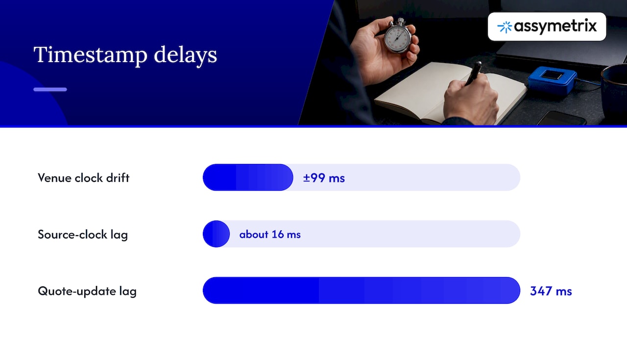
This is where most backtests quietly break. The OpenMarket dataset paper, which synchronizes Polymarket with Binance data for high-frequency research, found that venue clocks drift and lag: drift on the order of ±99 ms depending on venue, a persistent source-clock lag (about 16 ms median in their measurements), and a median 347 ms lag between a venue move and the Polymarket quote update. The authors’ conclusion is that assuming order-event creation times produces look-ahead bias, and that researchers should use venue-ingest timestamps.

What that means for your files:

• Always keep both ts_event and ts_ingest. You cannot recover the second one later.

• Simulate with ts_ingest. It reflects when your system could have known something. ts_event is useful for ordering within a venue, not for deciding what your strategy could see.

• Measure your own lag. Log the difference ts_ingest - ts_event per venue and plot its distribution. A fat tail is a warning that your sorted order is not your knowable order.

• Do not join cross-venue data on event time alone. Use an as-of join on ingest time with a tolerance window.

An as-of join in DuckDB:

SELECT a.ts_ingest, a.price AS poly_price, b.price AS kalshi_price
FROM poly a
ASOF JOIN kalshi b
  ON a.canonical_market_id = b.canonical_market_id
 AND a.ts_ingest >= b.ts_ingest;

SELECT a.ts_ingest, a.price AS poly_price, b.price AS kalshi_price
FROM poly a
ASOF JOIN kalshi b
  ON a.canonical_market_id = b.canonical_market_id
 AND a.ts_ingest >= b.ts_ingest;

Add a staleness filter afterwards (for example, drop pairs where the Kalshi quote is more than a few seconds old), or a spread that exists only because one side is stale will look like an opportunity.

From files to a backtest

A realistic backtest on Parquet history has four parts: a point-in-time view of prices (ingest-time ordered), a fee model, a fill model driven by order book depth rather than last price, and a resolution table that records how each market actually settled.

Fill assumptions matter more than signal sophistication. Real-time versus delayed data changes outcomes for short-horizon strategies, a point made well in this piece on why real-time market data decides short-term results, written for scalpers in other markets but equally true of thin prediction market books.

On arbitrage specifically, the TUM paper reports that some strategies, simulated over 800 days, exceeded 1000% returns in backtests. Treat that as an upper bound from idealized assumptions, not an expectation. Execution-aware fills, resolution-rule mismatches and stale quotes are what erode it. We walk through the mechanics in our prediction market arbitrage guide and a worked workflow in backtesting prediction market strategies with the Data API.

A short checklist before you trust a result

1. Does every row carry an ingest timestamp, and does the simulation use it?

2. Are venue-specific fees applied at the time of each trade?

3. Is each cross-venue pair confirmed to share resolution rules?

4. Do fills consume order book depth?

5. Are resolved and delisted markets included, so you avoid survivorship bias?

Feeding AI agents from Parquet

Agents rarely read raw Parquet, but they benefit from it indirectly. Parquet is the cold store from which you build features, calibration tables and retrieval snapshots. Live market prices then give the agent context at inference time.

The open-source market-edge project reports that blind LLM estimates were about 3.5 times worse than market-anchored ones, which supports using models as calibration layers on top of market prices rather than as standalone forecasters. A practical pattern: build a Parquet table of historical price versus final outcome by category, expose a summary tool to the agent, and feed it the current cross-venue price at decision time. Our guide to feeding prediction market data into an AI trading agent covers the live half of that loop.

Our perspective on Parquet and prediction market data

We build data infrastructure across Polymarket, Kalshi and Limitless, and the pattern we see from developers is consistent: the format debate is settled in an afternoon, while the identity and timing problems take months. Parquet is the correct storage layer. It does not tell you that two markets are the same question, and it does not tell you when your system could first have known a price.

That is why we treat canonical IDs and ingestion-time semantics as the product, with file format as a delivery detail. Our history covers roughly 1.5 terabytes and nearly one billion rows of trading activity, and a dataset of that size only stays reproducible if every row follows one schema from day one. Our advice to any team building its own archive: write the schema document first, store both clocks, and record resolution rules alongside prices. Neutrality across venues matters here too. A data layer tied to one exchange will tend to describe the world in that exchange’s terms.

— Dean

Skip the collection work

Building and maintaining a multi-venue archive means running collectors, repairing gaps and keeping schemas consistent as venues change. The Assymetrix Data API gives developers, quants and agents one integration for normalized, cross-venue real-time and historical data from Polymarket, Kalshi and Limitless, with bulk export for offline analysis. If you are sizing a research workload first, see our guide to the 1.5TB historical backfill.

FAQ

Is Parquet better than CSV for prediction market data?

For anything beyond small samples, yes. Parquet keeps column types, compresses repeated values heavily, and lets engines read only the columns and row groups a query needs. CSV remains fine for sharing a tiny sample or for quick inspection.

How should I partition Parquet files for Polymarket and Kalshi data?

Partition by venue and date, using Hive-style folders such as venue=kalshi/date=2026-10-19. Avoid partitioning by market ID, which creates many tiny files. Sort within files by canonical market ID and timestamp so row-group statistics can skip irrelevant data.

Which timestamp should I use for backtesting?

Use the time your system ingested each update, not the venue’s event time. Research on synchronized Polymarket data found venue clocks drift and lag, and that relying on event creation times introduces look-ahead bias. Store both columns so you can audit the difference.

Can I merge Parquet files with different schemas?

Yes, DuckDB’s union_by_name option unifies files whose columns differ. It is better to avoid the situation by enforcing one schema when data is ingested, so types and column names stay stable across venues and years.

Sources

• DuckDB: Parquet Tips

• DuckDB: Hive Partitioning

• Semantic Non-Fungibility and Violations of the Law of One Price in Prediction Markets (arXiv)

• OpenMarket: A Synchronized Polymarket-Binance Dataset (arXiv)

• datori/market-edge (GitHub)