Order Flow Analysis in Prediction Markets: A Quant Guide
Order Flow Analysis in Prediction Markets: A Quant Guide
Order Flow Analysis in Prediction Markets: A Quant Guide
Unlock insights with Order Flow Analysis in Prediction Markets. A Quant Guide reveals trade-level data to amplify your prediction strategies.
Order Flow Analysis in Prediction Markets: A Quant Guide
TL;DR:
Order flow analysis in prediction markets reveals execution patterns behind price moves and aids early detection of informed trades. Key signals include large-wallet entries, final hour volume spikes, and cross-venue positioning, all requiring precise, normalized trade data with strict resolution leakage controls. The Assymetrix Data API provides unified access to cross-venue trade data, enabling robust signal building and backtesting at scale.
Order flow analysis in prediction markets gives quant teams something price feeds cannot: the execution shape behind each move. Where a price chart shows what happened, trade-level data shows who acted, how they sized in, and when relative to resolution. The three highest-value advantages are identifying large-wallet concentration before a price shift, detecting informed flow in the final 30–60 minutes before resolution, and spotting cross-venue simultaneous positioning that confirms a directional thesis.
TL;DR: highest-impact signals to compute first
Large-wallet pre-resolution entries (wallet notional > 3× median in the last 60 minutes)
Last-hour volume spike (percent-volume in final 60 minutes vs. rolling 7-day baseline)
Buy/sell imbalance at structural price levels (Order Book Imbalance > +0.3 or < −0.3)
Cross-venue simultaneous buys on Polymarket and Kalshi within a 30-second window
Absorption at resting size (aggressive hits without price movement)
Wallet-concentration delta (top-5 wallet share change over a 4-hour window)
Immediate next steps: Subscribe to the Assymetrix WebSocket trade stream, pull a 30-day historical dump via the REST endpoint, and run a single SQL cumulative-delta query grouped by wallet_id and minutes_to_resolution. That is your starting backtest.
Table of Contents
Why does order flow behave differently in prediction markets?
What trade-level data do you need before building any signal?
Which order-flow signals should you compute first?
How do you design a reproducible backtest for these signals?
How do you build the ingestion pipeline from raw feed to features?
Where do you get normalized, cross-venue order-flow data?
Two reproducible examples: large-wallet detector and cross-venue spike synchrony
What are the most common failure modes for order-flow signals?
How do you combine order-flow signals with external fundamental data?
How do you exploit cross-venue order-flow discrepancies for arbitrage?
What statistical and machine learning models work best with order-flow inputs?
How do you handle cross-venue data inconsistencies and synchronization?
What open-source datasets and benchmark platforms exist for this research?
Key Takeaways
What actually matters when you productionize order-flow signals
Assymetrix gives you the data layer to start today
Useful sources
Why does order flow behave differently in prediction markets?
Three structural differences change how you build and interpret every signal.
1. Resolution deadlines create terminal flow. Equity momentum can persist indefinitely. Prediction market prices converge to 0 or 1 at a fixed date. That creates a resolution-driven flow regime: informed traders accumulate late, not early, because early positions carry more time risk. Frenzy Capital’s synthesis of academic literature confirms that last-minute movements accompanied by above-average volume strongly indicate informed participation, and recommends monitoring the final 30–60 minutes before resolution as a primary signal window.
2. Binary price bounds produce extreme boundary effects. Near 0 or near 1, books thin dramatically, spreads widen, and a small notional trade can move the price several cents. PredictEngine’s order-book analysis documents this boundary behavior and recommends multi-level depth aggregation and quote-refresh-rate monitoring as proxies for information arrival. A signal calibrated on mid-range liquidity will misfire badly near the extremes.
3. Wallet-level transparency on Polymarket vs. anonymized flow on Kalshi. Polymarket’s on-chain architecture exposes wallet addresses, letting you build wallet histories, label smart money, and track concentration. Kalshi’s centralized model anonymizes participants. Signal design must account for this asymmetry: wallet-based signals are native to Polymarket and Limitless; flow-aggregate signals (OBI, volume spike, cumulative delta) are the primary tools on Kalshi.
Dimension | Prediction markets | Equities/futures |
|---|---|---|
Venue transparency | Wallet-level (Polymarket/Limitless) or anonymized (Kalshi) | Anonymized, broker-aggregated |
Liquidity near price extremes | Thin, wide spreads, outsized impact | Relatively stable depth |
Settlement model | Binary, fixed-date resolution | Continuous, no forced settlement |
Market-making | Automated market makers or thin manual books | Designated market makers, HFT |
Informed-flow timing | Concentrates near resolution | Distributed across session |
The practical consequence: a signal that works in equities because it detects institutional accumulation over days needs to be compressed into hours or minutes for prediction markets, and the wallet-transparency layer on Polymarket lets you verify concentration directly rather than inferring it from aggregate tape.
What trade-level data do you need before building any signal?
The minimal schema for any order-flow signal has eleven fields. Missing even one of them forces you into approximations that degrade signal quality.
Minimum required fields per trade event:
event_id: canonical market identifier, normalized across venuestimestamp: nanosecond or microsecond precision; millisecond is the floor for cross-venue syncvenue: Polymarket, Kalshi, or Limitlessmarket_id: contract-level identifier within the eventcontract_side: YES or NO (binary outcome side)price: normalized to [0, 1] decimal, not cents or ticksquantity: shares or contracts, in a consistent unit per venuemaker_taker: aggressor flag where available (critical for absorption detection)wallet_id: pseudonymized address (Polymarket/Limitless) or null (Kalshi)order_type: market, limit, or AMM-fillorderbook_snapshot_id: foreign key to the book state at trade time
Data-quality checklist before you trust a feed:
Timestamp monotonicity: reject or flag out-of-order events within a venue
Missing-data tolerance: more than 0.5% null
wallet_idrows on Polymarket signals feed gapsWatermarking: tag late-arriving events with both event-time and processing-time so replay is deterministic
Price canonicalization: Kalshi may quote in cents; normalize to [0, 1] before any cross-venue join
Row-level provenance: each row should carry its source venue and ingestion batch ID for audit
Data dimension | Streaming (WebSocket) | Bulk historical |
|---|---|---|
Latency | Sub-second to a few seconds | Minutes to hours (batch export) |
Best use | Live signal generation, real-time alerts | Backtests, model training, replay |
Schema completeness | May drop orderbook snapshot fields | Full schema with provenance |
Retention | Rolling window (hours to days) | Full history (years) |
For live signal generation, WebSocket feeds are the only viable path. For backtests and model training, bulk historical exports with full provenance are preferable because they include the orderbook snapshot IDs needed for deterministic replay.
Which order-flow signals should you compute first?
Order-flow primitives — footprint charts, DOM, time-and-sales, and cumulative delta — reveal execution aggression and absorption. In prediction markets, eight signals deliver the highest return on implementation effort.
1. Large-wallet pre-resolution entry. A single wallet placing notional > 3× the 30-day median wallet trade size within 60 minutes of resolution. Parameterize by event category: political markets have different median sizes than sports markets.
2. Last-hour volume spike. Percent-volume in the final 60 minutes vs. a rolling 7-day baseline for the same market. A spike above 2× baseline with directional skew (>65% on one side) is a strong informed-flow flag.
3. Order Book Imbalance (OBI). (bid_volume_top_N - ask_volume_top_N) / (bid_volume_top_N + ask_volume_top_N). PredictEngine recommends OBI > +0.3 or < −0.3 as action thresholds, with N = 5 levels as a starting point. Near price boundaries, widen N to 10 to capture the thinner book.
4. Absorption at a structural level. Heavy aggressive flow (taker buys or sells) met by persistent resting size without price movement. TradeAlgo’s practitioner evidence confirms absorption confirmed at structural levels often precedes short-term reversals. Detection logic: taker_volume > 2× maker_replenishment_rate over a 5-minute window with price change < 0.5 cents.
5. Cumulative delta divergence. Running sum of (taker_buy_volume - taker_sell_volume) diverging from price direction. If price rises but cumulative delta turns negative, selling pressure is being absorbed, not reflected.
6. TWAP-style cadence. Regular, evenly-spaced trades of similar size from one or a small cluster of wallets. Kresmion’s detectors on Polymarket identify TWAP slices, absorption, and bid-ladder patterns as the three most common algorithmic execution shapes on public tape.
7. Cross-venue simultaneous positioning. The same directional trade appearing on Polymarket and Kalshi within a 30-second window, normalized for venue-specific price units. This is the highest-precision signal because it requires capital commitment on two separate systems.
8. Wallet-concentration delta. Change in the top-5 wallet share of open interest over a 4-hour rolling window. A concentration increase of > 10 percentage points without a corresponding price move often precedes a sharp directional shift.
Pro Tip: Treat detector outputs as structural flags, not directional calls. A TWAP pattern or absorption flag tells you that an algorithm is active; it does not tell you which way the market resolves. Always require a secondary signal (OBI direction, cumulative delta sign, cross-venue corroboration) before acting on a geometric flag alone.
A minimal SQL sketch for net flow by wallet:
SELECT
  wallet_id,
  SUM(CASE WHEN contract_side = 'YES' THEN quantity ELSE -quantity END) AS net_flow,
  SUM(quantity * price) AS notional,
  MIN(timestamp) AS first_trade,
  MAX(timestamp) AS last_trade
FROM trades
WHERE market_id = :market_id
  AND timestamp >= :window_start
GROUP BY wallet_id
ORDER BY ABS(net_flow) DESC;
SELECT
  wallet_id,
  SUM(CASE WHEN contract_side = 'YES' THEN quantity ELSE -quantity END) AS net_flow,
  SUM(quantity * price) AS notional,
  MIN(timestamp) AS first_trade,
  MAX(timestamp) AS last_trade
FROM trades
WHERE market_id = :market_id
  AND timestamp >= :window_start
GROUP BY wallet_id
ORDER BY ABS(net_flow) DESC;
How do you design a reproducible backtest for these signals?
The canonical replay approach: reconstruct the order book tick-by-tick from a historical event stream, apply a deterministic fill model, and evaluate signals against known resolution outcomes without any forward-looking data.
Replay checklist:
Slice the dataset by event date, not trade date, to prevent cross-event leakage.
Synchronize clocks across venues using UTC event-time timestamps; apply a 500ms tolerance for cross-venue joins.
Reconstruct the order book at each tick using the
orderbook_snapshot_idforeign key.Apply a deterministic matching rule: aggressive orders fill at the best available resting price at the moment of arrival; no partial-fill queue-priority assumptions unless your venue data includes queue position.
Mask all data from the final 60 seconds before resolution in training sets to prevent resolution leakage.
Handle partial fills by pro-rating notional at the fill price; never assume full fill on thin books.
Evaluation metrics:
Metric | Definition | Why it matters for prediction markets |
|---|---|---|
Hit rate by time-to-resolution bucket | Fraction of correct directional calls, binned by hours to resolution | Isolates whether signal degrades as resolution approaches |
P&L with slippage model | Net return after applying a 2-tick slippage assumption | Thin books make slippage material |
Precision/recall for signal windows | Standard classification metrics on flagged windows | Quantifies false-positive rate |
Bootstrap significance | bootstrap on P&L distribution | Guards against overfitting to a small event sample |
Frenzy Capital’s research and PredictEngine both emphasize cross-venue corroboration as a material precision booster. When a signal fires on both Polymarket and Kalshi within the same window, false-positive rates drop substantially compared to single-venue detection.
How do you build the ingestion pipeline from raw feed to features?
The minimal production pipeline has five stages: WebSocket ingestion → raw event log → canonicalization and enrichment → feature store → real-time signal engine.
Stage 1: WebSocket ingestion. Subscribe to per-market trade streams. Write every raw message to an append-only event log with processing-time watermarks. Never transform in-flight; log first, process second.
Stage 2: Canonicalization. Apply venue-specific price normalization (Kalshi cents → [0, 1] decimal), map venue-native market IDs to your canonical event_id, and pseudonymize wallet addresses with a stable hash. Tag each row with venue, event_time, and ingest_time.
Stage 3: Enrichment. Join to the orderbook snapshot table on orderbook_snapshot_id. Compute maker_taker where the venue does not supply it (infer from price-crossing logic). Attach minutes_to_resolution from your event calendar.
Stage 4: Feature store. Materialize sliding-window aggregates as views or pre-computed tables. A Python pseudocode sketch for sliding wallet notional:
def sliding_wallet_notional(trades_df, wallet_id, window_minutes=60):
    window = trades_df[
        (trades_df['wallet_id'] == wallet_id) &
        (trades_df['minutes_to_resolution'] <= window_minutes)
    ]
    return (window['quantity'] * window['price']).sum()
def sliding_wallet_notional(trades_df, wallet_id, window_minutes=60):
    window = trades_df[
        (trades_df['wallet_id'] == wallet_id) &
        (trades_df['minutes_to_resolution'] <= window_minutes)
    ]
    return (window['quantity'] * window['price']).sum()
Stage 5: Signal engine. Evaluate signal conditions against the feature store on each new trade event. Emit a structured signal record with signal_type, market_id, timestamp, confidence, and supporting_fields. Keep signal logic stateless where possible so replay is trivial.
For backtests, swap Stage 1 for a bulk historical export and replay events in timestamp order. The rest of the pipeline is identical, which is the point: production and backtest should share the same canonicalization and feature code. See the Assymetrix API integration guide for endpoint-level schema documentation.
Where do you get normalized, cross-venue order-flow data?
The Assymetrix Data API supplies trade-level events, wallet histories, normalized schemas, WebSocket real-time feeds, and bulk historical exports across Polymarket, Kalshi, and Limitless through a single integration. The dataset covers approximately 1.5 terabytes of historical data spanning nearly 900 million indexed events, with row-level provenance that makes deterministic replay tractable at scale.
What the API gives you directly:
Trade-level event stream with
wallet_id,price,quantity,side, andtimestampin a unified schemaWebSocket subscriptions per market or per venue for sub-second trade delivery
Bulk historical exports in Parquet or CSV for backtest ingestion
Smart Money wallet labels and Trader Skill Scores for wallet-concentration signals
Cross-venue arbitrage signals and market divergence alerts pre-computed
A minimal WebSocket subscription in Python:
import websockets, asyncio, json

async def stream_trades(market_id):
    uri = f"wss://data.assymetrix.com/v1/trades/{market_id}"
    async with websockets.connect(uri, extra_headers={"X-API-Key": API_KEY}) as ws:
        async for message in ws:
            event = json.loads(message)
            process_trade(event)  # canonicalize and write to event log
import websockets, asyncio, json

async def stream_trades(market_id):
    uri = f"wss://data.assymetrix.com/v1/trades/{market_id}"
    async with websockets.connect(uri, extra_headers={"X-API-Key": API_KEY}) as ws:
        async for message in ws:
            event = json.loads(message)
            process_trade(event)  # canonicalize and write to event log
Access tiers range from a free research tier (rate-limited, suitable for academic work and prototyping) to commercial tiers with full WebSocket throughput, bulk export access, and SLA-backed latency. The Python developer guide covers authentication, rate limits, and schema field definitions in detail.
Two reproducible examples: large-wallet detector and cross-venue spike synchrony
Example 1: Large-wallet pre-resolution entry detector.
Detection logic in one line: flag any wallet whose notional in the final 60 minutes exceeds 3× its own 30-day median trade size and whose direction matches a net OBI > +0.3.
def large_wallet_detector(trades, wallet_stats, obi, threshold_multiplier=3, window_min=60):
    recent = trades[trades['minutes_to_resolution'] <= window_min]
    for wallet_id, group in recent.groupby('wallet_id'):
        notional = (group['quantity'] * group['price']).sum()
        median_notional = wallet_stats.loc[wallet_id, 'median_30d_notional']
        direction = 'YES' if group['contract_side'].mode()[0] == 'YES' else 'NO'
        if notional > threshold_multiplier * median_notional and obi_aligned(obi, direction):
            emit_signal('LARGE_WALLET_ENTRY', wallet_id, notional, direction)
def large_wallet_detector(trades, wallet_stats, obi, threshold_multiplier=3, window_min=60):
    recent = trades[trades['minutes_to_resolution'] <= window_min]
    for wallet_id, group in recent.groupby('wallet_id'):
        notional = (group['quantity'] * group['price']).sum()
        median_notional = wallet_stats.loc[wallet_id, 'median_30d_notional']
        direction = 'YES' if group['contract_side'].mode()[0] == 'YES' else 'NO'
        if notional > threshold_multiplier * median_notional and obi_aligned(obi, direction):
            emit_signal('LARGE_WALLET_ENTRY', wallet_id, notional, direction)
Backtest assumptions: fill at mid-price at signal time, 2-tick slippage, no position held past resolution. Mask the final 60 seconds from training labels.
Example 2: Cross-venue spike synchrony detector.
Detection logic: flag when Polymarket and Kalshi both show a volume spike > 2× their respective 7-day baselines in the same direction within a 30-second window.
def cross_venue_spike(poly_trades, kalshi_trades, baseline, window_sec=30, spike_mult=2.0):
    for t in event_timestamps:
        poly_vol = volume_in_window(poly_trades, t, window_sec)
        kalshi_vol = volume_in_window(kalshi_trades, t, window_sec)
        poly_dir = net_direction(poly_trades, t, window_sec)
        kalshi_dir = net_direction(kalshi_trades, t, window_sec)
        if (poly_vol > spike_mult * baseline['poly'] and
            kalshi_vol > spike_mult * baseline['kalshi'] and
            poly_dir == kalshi_dir):
            emit_signal('CROSS_VENUE_SPIKE', t, poly_dir)
def cross_venue_spike(poly_trades, kalshi_trades, baseline, window_sec=30, spike_mult=2.0):
    for t in event_timestamps:
        poly_vol = volume_in_window(poly_trades, t, window_sec)
        kalshi_vol = volume_in_window(kalshi_trades, t, window_sec)
        poly_dir = net_direction(poly_trades, t, window_sec)
        kalshi_dir = net_direction(kalshi_trades, t, window_sec)
        if (poly_vol > spike_mult * baseline['poly'] and
            kalshi_vol > spike_mult * baseline['kalshi'] and
            poly_dir == kalshi_dir):
            emit_signal('CROSS_VENUE_SPIKE', t, poly_dir)
Pro Tip: For the cross-venue detector, randomize wall-clock offsets by ±5 seconds in bootstrap runs to test whether the 30-second synchrony window is genuinely informative or an artifact of your clock-alignment assumptions. If precision drops sharply at ±10 seconds, the signal is real. If it holds flat, you are likely detecting correlated retail flow, not informed positioning.
Robustness checklist: run bootstrap windows of 500 and 2,000 iterations, scale volume thresholds by venue-normalized median depth, and always evaluate on a holdout split by event date (never by trade date).
What are the most common failure modes for order-flow signals?
Six pitfalls destroy naive order-flow signals in prediction markets before they reach production.
Resolution leakage. Including any data from the final 60 seconds before resolution in training labels inflates hit rates artificially. Mask this window unconditionally.
Survivorship bias. Building signals only on markets that resolved with high volume excludes the thin, ambiguous markets where false positives are most damaging.
Wallet reuse and clustering. A single actor operating multiple wallets can appear as broad-based accumulation. Cluster wallets by behavioral similarity (trade timing, size distribution, co-occurrence) before computing concentration metrics.
Thin-market noise. On markets with median depth < 500 shares, a single retail trade can trigger an OBI > +0.3 flag. Require a minimum depth threshold before any OBI signal fires.
Base-rate neglect. Kresmion’s Bayesian analysis shows that even a high-sensitivity detector produces many false positives when the true-event base rate is low. A detector with 90% sensitivity and a 5% false-positive rate can have precision around 27% when genuine algorithmic events occur in only 2% of windows. Always compute precision, not just recall.
Crowd-flow contamination. Pre-resolution retail herding produces volume spikes that mimic informed flow. Require cross-venue corroboration or wallet-concentration confirmation before treating a spike as informed.
Validation checklist before trusting a signal:
Compute volume-normalized effect sizes; raw notional is misleading across markets of different sizes.
Hold out by event type (political, sports, economic) and verify the signal generalizes.
Run wallet-aggregation sensitivity: does the signal survive if you merge wallets within 2 hops of a common funding source?
Verify cross-venue timing consistency within a ±30-second tolerance.
Confirm the signal fires on at least 20 distinct events before reporting precision metrics.
Red flags that warrant rejection: signal fires only on one wallet in the entire history, cross-venue timing is inconsistent by more than 60 seconds, or the effect disappears when you apply a 2-tick slippage model.
How do you combine order-flow signals with external fundamental data?
Order-flow signals are strongest when anchored to an event calendar. Combining them with external data reduces false positives from retail crowd activity and improves precision on genuinely informed flow.
The most productive integration pattern is a two-layer model: the first layer scores each trade event on structural order-flow features (OBI, wallet concentration, cumulative delta); the second layer gates those scores against an event-context feature set derived from external sources. Event-context features include time-to-announcement for scheduled events (Fed decisions, election dates, earnings), news-sentiment scores from sources like GDELT or Bloomberg Terminal feeds, and historical base rates for the specific event type.
For political markets, polling averages from FiveThirtyEight or RealClearPolitics provide a prior probability that sharpens the interpretation of late flow. A large-wallet YES entry on a market already priced at 0.85 carries different information than the same entry on a market at 0.50. Conditioning on the prior prevents the model from over-weighting flow that is simply tracking a consensus shift.
The practical implementation: join your feature store to an event-metadata table on event_id, and compute interaction features like wallet_notional × (1 - current_price) (the implied information value of a late YES entry) and volume_spike_ratio × days_to_resolution. These interaction terms consistently outperform raw order-flow features in cross-validated evaluation on prediction-market data.
How do you exploit cross-venue order-flow discrepancies for arbitrage?
Cross-venue arbitrage in prediction markets operates on two distinct edges: price discrepancies and flow-timing discrepancies. Price discrepancies are well-known and arbitraged quickly. Flow-timing discrepancies are less crowded and more durable.
A flow-timing discrepancy occurs when informed flow appears on one venue before the other. On Polymarket, on-chain settlement creates a slight execution delay relative to Kalshi’s centralized matching. A large-wallet entry on Polymarket that has not yet moved the Kalshi price creates a short window (typically 10–60 seconds) to position on Kalshi before the price converges. Detecting this requires sub-second timestamp alignment across venues and a pre-computed price-equivalence mapping that accounts for Kalshi’s cent-based quoting.
The cross-venue signal generation guide covers the normalization steps in detail. The key operational requirement is a shared event clock: both venue feeds must be watermarked to the same UTC reference before any cross-venue join. A 500ms clock skew can turn a genuine 30-second arbitrage window into noise.
For structural arbitrage (persistent price gaps rather than flow-timing edges), the standard approach is a pairs model: compute the historical spread between Polymarket and Kalshi prices for the same underlying event, fit a mean-reversion model, and trade when the spread exceeds 2 standard deviations. Order-flow signals add value here as an entry filter: enter the spread trade only when the flow on the cheaper venue is directionally consistent with the spread closing, not widening.
What statistical and machine learning models work best with order-flow inputs?
Prediction-market order-flow data has three properties that constrain model choice: small event counts (hundreds to low thousands of resolved markets), high within-event autocorrelation (trades cluster near resolution), and a binary outcome label.
Gradient-boosted trees (XGBoost, LightGBM) handle the tabular feature set well and are robust to the class imbalance typical of informed-flow labels. Feature engineering for tree models: compute rolling statistics at multiple windows (5-minute, 30-minute, 60-minute), include minutes_to_resolution as a raw feature and as an interaction term with every flow metric, and add venue-normalized versions of all volume features.
Logistic regression with regularization remains a strong baseline for binary outcome prediction when the event count is low. It is interpretable, fast to retrain, and less prone to overfitting than deep models on small samples. Use L2 regularization and standardize all features before fitting.
Sequence models (LSTM, Transformer) are worth exploring for the trade-event stream itself, treating each market as a variable-length sequence of trade events. The practical constraint is data volume: a Transformer trained on fewer than 500 resolved markets will overfit unless you apply aggressive dropout and early stopping. Pre-training on a larger corpus of markets (using Assymetrix’s ~900M event dataset) and fine-tuning on a specific event category is a more tractable approach.
Feature engineering priorities: the most predictive features across model types are wallet_concentration_delta_4h, last_60min_volume_pct, cross_venue_sync_flag, and obi_at_signal_time. Interaction features between minutes_to_resolution and flow metrics consistently rank in the top quartile of feature importance.
How do you handle cross-venue data inconsistencies and synchronization?
Three categories of inconsistency require explicit handling before any cross-venue analysis: schema divergence, clock skew, and liquidity-unit mismatches.
Schema divergence is the most common. Polymarket uses on-chain token addresses as market identifiers; Kalshi uses human-readable ticker strings; Limitless uses its own internal IDs. A canonical event_id mapping table, maintained as a lookup service, is the only reliable solution. Map every venue-native ID to a canonical event on ingest, not at query time.
Clock skew between venues can reach several seconds under normal conditions and tens of seconds during high-load periods. The correct approach is to watermark every event with both event_time (the venue’s reported timestamp) and ingest_time (your system’s receipt time), then use event_time for all cross-venue joins with a configurable tolerance (500ms for tight synchrony checks, 5 seconds for looser correlation analysis).
Liquidity-unit mismatches arise because Kalshi quotes in cents and Polymarket quotes in fractional dollars. Normalize all prices to [0, 1] decimal before any join or comparison. Volume units also differ: Polymarket reports shares, Kalshi reports contracts. Maintain a per-venue unit-conversion table and apply it at canonicalization time.
A practical test for synchronization quality: compute the cross-venue price correlation for the same event at 1-second, 5-second, and 30-second lags. If correlation peaks at a non-zero lag, your clock alignment has a systematic offset that needs correction before cross-venue signals will be reliable.
What open-source datasets and benchmark platforms exist for this research?
The honest answer is that prediction-market order-flow research lacks the standardized benchmark datasets that equity microstructure research enjoys. Most public data is price-only or low-frequency.
Polymarket’s on-chain data is the most accessible raw source. Because all trades settle on Polygon, the full trade history is queryable via the Polygon blockchain explorer or via Polymarket’s public subgraph (The Graph protocol). The limitation is that raw on-chain data requires significant normalization work: you must reconstruct market IDs, map contract addresses to human-readable events, and handle AMM-fill events separately from limit-order fills.
Kalshi does not publish trade-level data publicly. Its API provides market prices and volume aggregates but not individual trade records or wallet-equivalent identifiers.
Limitless is newer and has limited public data infrastructure at this stage.
For standardized research, the most practical path is Assymetrix’s research tier, which provides normalized, cross-venue trade-level data with row-level provenance. The Assymetrix backtesting guide documents how to use historical exports for reproducible experiments. For academic teams, a non-commercial research license is available.
On the open-source tooling side, the Augur v2 dataset (Ethereum-based prediction market, now largely inactive) has been used in several published microstructure papers and provides a useful benchmark for signal validation methodology, even though the venue is no longer active.
Key Takeaways
Order-flow analysis in prediction markets delivers its highest value when you instrument wallet-level signals, enforce strict resolution-leakage controls, and corroborate single-venue flags with cross-venue data before acting.
Point | Details |
|---|---|
Instrument WebSocket first | Subscribe to real-time trade streams before building any model; live data reveals signal decay that backtests miss. |
Last-hour flow is the primary window | Informed traders concentrate near resolution; monitor the final 60 minutes with volume-normalized metrics. |
Cross-venue corroboration cuts false positives | Require simultaneous signals on Polymarket and Kalshi within a 30-second window to confirm informed flow. |
Mask the final 60 seconds in training | Resolution leakage is the single most common cause of inflated backtest hit rates; enforce this unconditionally. |
Assymetrix provides the unified feed | The Assymetrix Data API covers ~1.5 TB and ~900M indexed events across Polymarket, Kalshi, and Limitless with wallet histories and pre-computed Smart Money labels. |
What actually matters when you productionize order-flow signals
The conventional wisdom in quant research is to spend most of your time on model sophistication. For prediction-market order flow, that priority is inverted. The bottleneck is almost never the model; it is the reliability of the signal infrastructure underneath it.
A team that instruments a clean WebSocket feed, enforces strict clock synchronization, and runs a simple logistic regression on five well-defined features will outperform a team running a Transformer on a noisy, poorly-normalized feed. The resolution-driven microstructure of prediction markets means that signal windows are short, data is sparse, and a single bad event in your training set can corrupt an entire model generation. Provenance matters more here than in equity research.
Operationally, set a latency SLA for your signal engine before you set a performance target. If your WebSocket-to-signal latency exceeds 5 seconds, you are already outside the actionable window for last-hour informed-flow signals on thin markets. Monitor for concept drift around event calendars: political markets in election cycles behave differently from off-cycle political markets, and a model trained on one regime will degrade in the other.
The near-term roadmap for most teams should be: (1) instrument the feed and validate schema completeness, (2) compute the eight signals from Section 4 and measure their raw precision on a holdout set, (3) add cross-venue corroboration as a filter, and (4) only then introduce a learned model on top of the validated signal layer. Skipping steps 1 through 3 is the most common reason prediction-market quant projects stall.
Assymetrix gives you the data layer to start today
Getting normalized, cross-venue order-flow data with WebSocket streaming and bulk historical exports used to require building separate integrations for each venue. Assymetrix collapses that into a single API call.
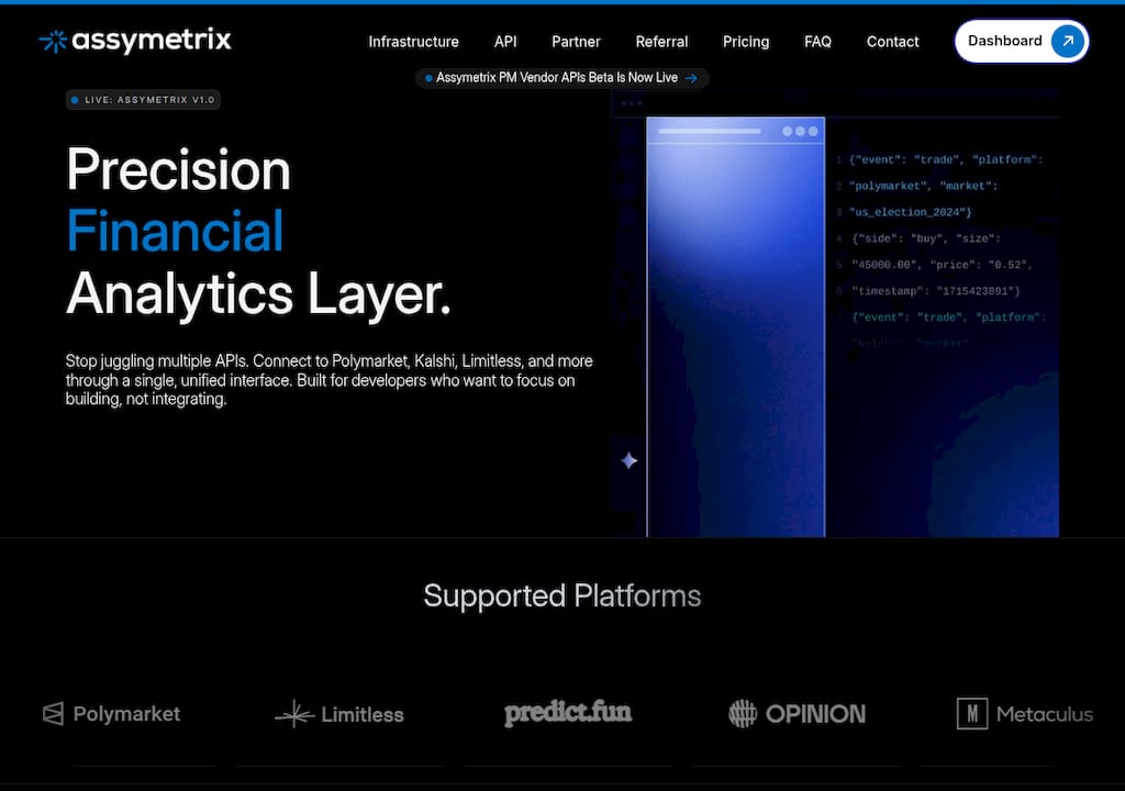
The Assymetrix Data API covers Polymarket, Kalshi, and Limitless in a unified schema, with approximately 1.5 TB of historical trade-level data and nearly 900 million indexed events available for replay and model training. Smart Money wallet labels and Trader Skill Scores are pre-computed, so you can skip the wallet-clustering work and go straight to signal validation. Access tiers include a free research tier for prototyping and academic use, with commercial tiers for production throughput and SLA-backed latency. For teams building cross-venue arbitrage strategies, the prediction market arbitrage guide covers the normalization and signal-generation steps in detail. Request API access or review the full endpoint documentation at data.assymetrix.com.
Useful sources
Algorithmic Footprints in Prediction Markets: How to Spot Execution Algorithms in the Public Tape | Kresmion Research
Order Flow Trading 2026 — Read the Footprint of Institutions
Order Book Analysis for Prediction Markets: $10K Guide | PredictEngine | PredictEngine
Order Flow Analysis: How to Read the Tape Like a Professional Trader | TradeAlgo
Ten Empirically-Grounded Prediction Market Trading Strategies — Frenzy Capital
Assymetrix | Prediction Markets Intelligence
FAQ
What is order flow analysis in prediction markets?
Order flow analysis examines individual trade events, wallet activity, and order-book dynamics to identify who is buying or selling, at what size, and when relative to resolution. It reveals execution patterns that price-only signals cannot capture.
How does prediction-market order flow differ from equity order flow?
Prediction markets have binary price bounds, resolution deadlines that concentrate informed flow near expiry, and wallet-level transparency on venues like Polymarket. Equity order flow is anonymous, continuous, and momentum-driven rather than resolution-driven.
What is the most reliable signal for detecting informed flow before resolution?
Frenzy Capital’s synthesis of academic literature identifies last-hour volume spikes accompanied by above-average directional skew as the strongest informed-flow indicator, especially when corroborated by cross-venue simultaneous positioning.
How do you avoid resolution leakage in a prediction-market backtest?
Mask all data from the final 60 seconds before resolution in training labels, slice your evaluation set by event date rather than trade date, and never include resolution outcomes as features in any model trained on pre-resolution data.
Where can you access normalized, trade-level prediction-market data for research?
The Assymetrix Data API at data.assymetrix.com provides cross-venue trade-level data across Polymarket, Kalshi, and Limitless, with approximately 1.5 TB of historical data and nearly 900 million indexed events available under research and commercial tiers.
Order Flow Analysis in Prediction Markets: A Quant Guide
TL;DR:
Order flow analysis in prediction markets reveals execution patterns behind price moves and aids early detection of informed trades. Key signals include large-wallet entries, final hour volume spikes, and cross-venue positioning, all requiring precise, normalized trade data with strict resolution leakage controls. The Assymetrix Data API provides unified access to cross-venue trade data, enabling robust signal building and backtesting at scale.
Order flow analysis in prediction markets gives quant teams something price feeds cannot: the execution shape behind each move. Where a price chart shows what happened, trade-level data shows who acted, how they sized in, and when relative to resolution. The three highest-value advantages are identifying large-wallet concentration before a price shift, detecting informed flow in the final 30–60 minutes before resolution, and spotting cross-venue simultaneous positioning that confirms a directional thesis.
TL;DR: highest-impact signals to compute first
Large-wallet pre-resolution entries (wallet notional > 3× median in the last 60 minutes)
Last-hour volume spike (percent-volume in final 60 minutes vs. rolling 7-day baseline)
Buy/sell imbalance at structural price levels (Order Book Imbalance > +0.3 or < −0.3)
Cross-venue simultaneous buys on Polymarket and Kalshi within a 30-second window
Absorption at resting size (aggressive hits without price movement)
Wallet-concentration delta (top-5 wallet share change over a 4-hour window)
Immediate next steps: Subscribe to the Assymetrix WebSocket trade stream, pull a 30-day historical dump via the REST endpoint, and run a single SQL cumulative-delta query grouped by wallet_id and minutes_to_resolution. That is your starting backtest.
Table of Contents
Why does order flow behave differently in prediction markets?
What trade-level data do you need before building any signal?
Which order-flow signals should you compute first?
How do you design a reproducible backtest for these signals?
How do you build the ingestion pipeline from raw feed to features?
Where do you get normalized, cross-venue order-flow data?
Two reproducible examples: large-wallet detector and cross-venue spike synchrony
What are the most common failure modes for order-flow signals?
How do you combine order-flow signals with external fundamental data?
How do you exploit cross-venue order-flow discrepancies for arbitrage?
What statistical and machine learning models work best with order-flow inputs?
How do you handle cross-venue data inconsistencies and synchronization?
What open-source datasets and benchmark platforms exist for this research?
Key Takeaways
What actually matters when you productionize order-flow signals
Assymetrix gives you the data layer to start today
Useful sources
Why does order flow behave differently in prediction markets?
Three structural differences change how you build and interpret every signal.
1. Resolution deadlines create terminal flow. Equity momentum can persist indefinitely. Prediction market prices converge to 0 or 1 at a fixed date. That creates a resolution-driven flow regime: informed traders accumulate late, not early, because early positions carry more time risk. Frenzy Capital’s synthesis of academic literature confirms that last-minute movements accompanied by above-average volume strongly indicate informed participation, and recommends monitoring the final 30–60 minutes before resolution as a primary signal window.
2. Binary price bounds produce extreme boundary effects. Near 0 or near 1, books thin dramatically, spreads widen, and a small notional trade can move the price several cents. PredictEngine’s order-book analysis documents this boundary behavior and recommends multi-level depth aggregation and quote-refresh-rate monitoring as proxies for information arrival. A signal calibrated on mid-range liquidity will misfire badly near the extremes.
3. Wallet-level transparency on Polymarket vs. anonymized flow on Kalshi. Polymarket’s on-chain architecture exposes wallet addresses, letting you build wallet histories, label smart money, and track concentration. Kalshi’s centralized model anonymizes participants. Signal design must account for this asymmetry: wallet-based signals are native to Polymarket and Limitless; flow-aggregate signals (OBI, volume spike, cumulative delta) are the primary tools on Kalshi.
Dimension | Prediction markets | Equities/futures |
|---|---|---|
Venue transparency | Wallet-level (Polymarket/Limitless) or anonymized (Kalshi) | Anonymized, broker-aggregated |
Liquidity near price extremes | Thin, wide spreads, outsized impact | Relatively stable depth |
Settlement model | Binary, fixed-date resolution | Continuous, no forced settlement |
Market-making | Automated market makers or thin manual books | Designated market makers, HFT |
Informed-flow timing | Concentrates near resolution | Distributed across session |
The practical consequence: a signal that works in equities because it detects institutional accumulation over days needs to be compressed into hours or minutes for prediction markets, and the wallet-transparency layer on Polymarket lets you verify concentration directly rather than inferring it from aggregate tape.
What trade-level data do you need before building any signal?
The minimal schema for any order-flow signal has eleven fields. Missing even one of them forces you into approximations that degrade signal quality.
Minimum required fields per trade event:
event_id: canonical market identifier, normalized across venuestimestamp: nanosecond or microsecond precision; millisecond is the floor for cross-venue syncvenue: Polymarket, Kalshi, or Limitlessmarket_id: contract-level identifier within the eventcontract_side: YES or NO (binary outcome side)price: normalized to [0, 1] decimal, not cents or ticksquantity: shares or contracts, in a consistent unit per venuemaker_taker: aggressor flag where available (critical for absorption detection)wallet_id: pseudonymized address (Polymarket/Limitless) or null (Kalshi)order_type: market, limit, or AMM-fillorderbook_snapshot_id: foreign key to the book state at trade time
Data-quality checklist before you trust a feed:
Timestamp monotonicity: reject or flag out-of-order events within a venue
Missing-data tolerance: more than 0.5% null
wallet_idrows on Polymarket signals feed gapsWatermarking: tag late-arriving events with both event-time and processing-time so replay is deterministic
Price canonicalization: Kalshi may quote in cents; normalize to [0, 1] before any cross-venue join
Row-level provenance: each row should carry its source venue and ingestion batch ID for audit
Data dimension | Streaming (WebSocket) | Bulk historical |
|---|---|---|
Latency | Sub-second to a few seconds | Minutes to hours (batch export) |
Best use | Live signal generation, real-time alerts | Backtests, model training, replay |
Schema completeness | May drop orderbook snapshot fields | Full schema with provenance |
Retention | Rolling window (hours to days) | Full history (years) |
For live signal generation, WebSocket feeds are the only viable path. For backtests and model training, bulk historical exports with full provenance are preferable because they include the orderbook snapshot IDs needed for deterministic replay.
Which order-flow signals should you compute first?
Order-flow primitives — footprint charts, DOM, time-and-sales, and cumulative delta — reveal execution aggression and absorption. In prediction markets, eight signals deliver the highest return on implementation effort.
1. Large-wallet pre-resolution entry. A single wallet placing notional > 3× the 30-day median wallet trade size within 60 minutes of resolution. Parameterize by event category: political markets have different median sizes than sports markets.
2. Last-hour volume spike. Percent-volume in the final 60 minutes vs. a rolling 7-day baseline for the same market. A spike above 2× baseline with directional skew (>65% on one side) is a strong informed-flow flag.
3. Order Book Imbalance (OBI). (bid_volume_top_N - ask_volume_top_N) / (bid_volume_top_N + ask_volume_top_N). PredictEngine recommends OBI > +0.3 or < −0.3 as action thresholds, with N = 5 levels as a starting point. Near price boundaries, widen N to 10 to capture the thinner book.
4. Absorption at a structural level. Heavy aggressive flow (taker buys or sells) met by persistent resting size without price movement. TradeAlgo’s practitioner evidence confirms absorption confirmed at structural levels often precedes short-term reversals. Detection logic: taker_volume > 2× maker_replenishment_rate over a 5-minute window with price change < 0.5 cents.
5. Cumulative delta divergence. Running sum of (taker_buy_volume - taker_sell_volume) diverging from price direction. If price rises but cumulative delta turns negative, selling pressure is being absorbed, not reflected.
6. TWAP-style cadence. Regular, evenly-spaced trades of similar size from one or a small cluster of wallets. Kresmion’s detectors on Polymarket identify TWAP slices, absorption, and bid-ladder patterns as the three most common algorithmic execution shapes on public tape.
7. Cross-venue simultaneous positioning. The same directional trade appearing on Polymarket and Kalshi within a 30-second window, normalized for venue-specific price units. This is the highest-precision signal because it requires capital commitment on two separate systems.
8. Wallet-concentration delta. Change in the top-5 wallet share of open interest over a 4-hour rolling window. A concentration increase of > 10 percentage points without a corresponding price move often precedes a sharp directional shift.
Pro Tip: Treat detector outputs as structural flags, not directional calls. A TWAP pattern or absorption flag tells you that an algorithm is active; it does not tell you which way the market resolves. Always require a secondary signal (OBI direction, cumulative delta sign, cross-venue corroboration) before acting on a geometric flag alone.
A minimal SQL sketch for net flow by wallet:
SELECT
  wallet_id,
  SUM(CASE WHEN contract_side = 'YES' THEN quantity ELSE -quantity END) AS net_flow,
  SUM(quantity * price) AS notional,
  MIN(timestamp) AS first_trade,
  MAX(timestamp) AS last_trade
FROM trades
WHERE market_id = :market_id
  AND timestamp >= :window_start
GROUP BY wallet_id
ORDER BY ABS(net_flow) DESC;
How do you design a reproducible backtest for these signals?
The canonical replay approach: reconstruct the order book tick-by-tick from a historical event stream, apply a deterministic fill model, and evaluate signals against known resolution outcomes without any forward-looking data.
Replay checklist:
Slice the dataset by event date, not trade date, to prevent cross-event leakage.
Synchronize clocks across venues using UTC event-time timestamps; apply a 500ms tolerance for cross-venue joins.
Reconstruct the order book at each tick using the
orderbook_snapshot_idforeign key.Apply a deterministic matching rule: aggressive orders fill at the best available resting price at the moment of arrival; no partial-fill queue-priority assumptions unless your venue data includes queue position.
Mask all data from the final 60 seconds before resolution in training sets to prevent resolution leakage.
Handle partial fills by pro-rating notional at the fill price; never assume full fill on thin books.
Evaluation metrics:
Metric | Definition | Why it matters for prediction markets |
|---|---|---|
Hit rate by time-to-resolution bucket | Fraction of correct directional calls, binned by hours to resolution | Isolates whether signal degrades as resolution approaches |
P&L with slippage model | Net return after applying a 2-tick slippage assumption | Thin books make slippage material |
Precision/recall for signal windows | Standard classification metrics on flagged windows | Quantifies false-positive rate |
Bootstrap significance | bootstrap on P&L distribution | Guards against overfitting to a small event sample |
Frenzy Capital’s research and PredictEngine both emphasize cross-venue corroboration as a material precision booster. When a signal fires on both Polymarket and Kalshi within the same window, false-positive rates drop substantially compared to single-venue detection.
How do you build the ingestion pipeline from raw feed to features?
The minimal production pipeline has five stages: WebSocket ingestion → raw event log → canonicalization and enrichment → feature store → real-time signal engine.
Stage 1: WebSocket ingestion. Subscribe to per-market trade streams. Write every raw message to an append-only event log with processing-time watermarks. Never transform in-flight; log first, process second.
Stage 2: Canonicalization. Apply venue-specific price normalization (Kalshi cents → [0, 1] decimal), map venue-native market IDs to your canonical event_id, and pseudonymize wallet addresses with a stable hash. Tag each row with venue, event_time, and ingest_time.
Stage 3: Enrichment. Join to the orderbook snapshot table on orderbook_snapshot_id. Compute maker_taker where the venue does not supply it (infer from price-crossing logic). Attach minutes_to_resolution from your event calendar.
Stage 4: Feature store. Materialize sliding-window aggregates as views or pre-computed tables. A Python pseudocode sketch for sliding wallet notional:
def sliding_wallet_notional(trades_df, wallet_id, window_minutes=60):
    window = trades_df[
        (trades_df['wallet_id'] == wallet_id) &
        (trades_df['minutes_to_resolution'] <= window_minutes)
    ]
    return (window['quantity'] * window['price']).sum()
Stage 5: Signal engine. Evaluate signal conditions against the feature store on each new trade event. Emit a structured signal record with signal_type, market_id, timestamp, confidence, and supporting_fields. Keep signal logic stateless where possible so replay is trivial.
For backtests, swap Stage 1 for a bulk historical export and replay events in timestamp order. The rest of the pipeline is identical, which is the point: production and backtest should share the same canonicalization and feature code. See the Assymetrix API integration guide for endpoint-level schema documentation.
Where do you get normalized, cross-venue order-flow data?
The Assymetrix Data API supplies trade-level events, wallet histories, normalized schemas, WebSocket real-time feeds, and bulk historical exports across Polymarket, Kalshi, and Limitless through a single integration. The dataset covers approximately 1.5 terabytes of historical data spanning nearly 900 million indexed events, with row-level provenance that makes deterministic replay tractable at scale.
What the API gives you directly:
Trade-level event stream with
wallet_id,price,quantity,side, andtimestampin a unified schemaWebSocket subscriptions per market or per venue for sub-second trade delivery
Bulk historical exports in Parquet or CSV for backtest ingestion
Smart Money wallet labels and Trader Skill Scores for wallet-concentration signals
Cross-venue arbitrage signals and market divergence alerts pre-computed
A minimal WebSocket subscription in Python:
import websockets, asyncio, json

async def stream_trades(market_id):
    uri = f"wss://data.assymetrix.com/v1/trades/{market_id}"
    async with websockets.connect(uri, extra_headers={"X-API-Key": API_KEY}) as ws:
        async for message in ws:
            event = json.loads(message)
            process_trade(event)  # canonicalize and write to event log
Access tiers range from a free research tier (rate-limited, suitable for academic work and prototyping) to commercial tiers with full WebSocket throughput, bulk export access, and SLA-backed latency. The Python developer guide covers authentication, rate limits, and schema field definitions in detail.
Two reproducible examples: large-wallet detector and cross-venue spike synchrony
Example 1: Large-wallet pre-resolution entry detector.
Detection logic in one line: flag any wallet whose notional in the final 60 minutes exceeds 3× its own 30-day median trade size and whose direction matches a net OBI > +0.3.
def large_wallet_detector(trades, wallet_stats, obi, threshold_multiplier=3, window_min=60):
    recent = trades[trades['minutes_to_resolution'] <= window_min]
    for wallet_id, group in recent.groupby('wallet_id'):
        notional = (group['quantity'] * group['price']).sum()
        median_notional = wallet_stats.loc[wallet_id, 'median_30d_notional']
        direction = 'YES' if group['contract_side'].mode()[0] == 'YES' else 'NO'
        if notional > threshold_multiplier * median_notional and obi_aligned(obi, direction):
            emit_signal('LARGE_WALLET_ENTRY', wallet_id, notional, direction)
Backtest assumptions: fill at mid-price at signal time, 2-tick slippage, no position held past resolution. Mask the final 60 seconds from training labels.
Example 2: Cross-venue spike synchrony detector.
Detection logic: flag when Polymarket and Kalshi both show a volume spike > 2× their respective 7-day baselines in the same direction within a 30-second window.
def cross_venue_spike(poly_trades, kalshi_trades, baseline, window_sec=30, spike_mult=2.0):
    for t in event_timestamps:
        poly_vol = volume_in_window(poly_trades, t, window_sec)
        kalshi_vol = volume_in_window(kalshi_trades, t, window_sec)
        poly_dir = net_direction(poly_trades, t, window_sec)
        kalshi_dir = net_direction(kalshi_trades, t, window_sec)
        if (poly_vol > spike_mult * baseline['poly'] and
            kalshi_vol > spike_mult * baseline['kalshi'] and
            poly_dir == kalshi_dir):
            emit_signal('CROSS_VENUE_SPIKE', t, poly_dir)
Pro Tip: For the cross-venue detector, randomize wall-clock offsets by ±5 seconds in bootstrap runs to test whether the 30-second synchrony window is genuinely informative or an artifact of your clock-alignment assumptions. If precision drops sharply at ±10 seconds, the signal is real. If it holds flat, you are likely detecting correlated retail flow, not informed positioning.
Robustness checklist: run bootstrap windows of 500 and 2,000 iterations, scale volume thresholds by venue-normalized median depth, and always evaluate on a holdout split by event date (never by trade date).
What are the most common failure modes for order-flow signals?
Six pitfalls destroy naive order-flow signals in prediction markets before they reach production.
Resolution leakage. Including any data from the final 60 seconds before resolution in training labels inflates hit rates artificially. Mask this window unconditionally.
Survivorship bias. Building signals only on markets that resolved with high volume excludes the thin, ambiguous markets where false positives are most damaging.
Wallet reuse and clustering. A single actor operating multiple wallets can appear as broad-based accumulation. Cluster wallets by behavioral similarity (trade timing, size distribution, co-occurrence) before computing concentration metrics.
Thin-market noise. On markets with median depth < 500 shares, a single retail trade can trigger an OBI > +0.3 flag. Require a minimum depth threshold before any OBI signal fires.
Base-rate neglect. Kresmion’s Bayesian analysis shows that even a high-sensitivity detector produces many false positives when the true-event base rate is low. A detector with 90% sensitivity and a 5% false-positive rate can have precision around 27% when genuine algorithmic events occur in only 2% of windows. Always compute precision, not just recall.
Crowd-flow contamination. Pre-resolution retail herding produces volume spikes that mimic informed flow. Require cross-venue corroboration or wallet-concentration confirmation before treating a spike as informed.
Validation checklist before trusting a signal:
Compute volume-normalized effect sizes; raw notional is misleading across markets of different sizes.
Hold out by event type (political, sports, economic) and verify the signal generalizes.
Run wallet-aggregation sensitivity: does the signal survive if you merge wallets within 2 hops of a common funding source?
Verify cross-venue timing consistency within a ±30-second tolerance.
Confirm the signal fires on at least 20 distinct events before reporting precision metrics.
Red flags that warrant rejection: signal fires only on one wallet in the entire history, cross-venue timing is inconsistent by more than 60 seconds, or the effect disappears when you apply a 2-tick slippage model.
How do you combine order-flow signals with external fundamental data?
Order-flow signals are strongest when anchored to an event calendar. Combining them with external data reduces false positives from retail crowd activity and improves precision on genuinely informed flow.
The most productive integration pattern is a two-layer model: the first layer scores each trade event on structural order-flow features (OBI, wallet concentration, cumulative delta); the second layer gates those scores against an event-context feature set derived from external sources. Event-context features include time-to-announcement for scheduled events (Fed decisions, election dates, earnings), news-sentiment scores from sources like GDELT or Bloomberg Terminal feeds, and historical base rates for the specific event type.
For political markets, polling averages from FiveThirtyEight or RealClearPolitics provide a prior probability that sharpens the interpretation of late flow. A large-wallet YES entry on a market already priced at 0.85 carries different information than the same entry on a market at 0.50. Conditioning on the prior prevents the model from over-weighting flow that is simply tracking a consensus shift.
The practical implementation: join your feature store to an event-metadata table on event_id, and compute interaction features like wallet_notional × (1 - current_price) (the implied information value of a late YES entry) and volume_spike_ratio × days_to_resolution. These interaction terms consistently outperform raw order-flow features in cross-validated evaluation on prediction-market data.
How do you exploit cross-venue order-flow discrepancies for arbitrage?
Cross-venue arbitrage in prediction markets operates on two distinct edges: price discrepancies and flow-timing discrepancies. Price discrepancies are well-known and arbitraged quickly. Flow-timing discrepancies are less crowded and more durable.
A flow-timing discrepancy occurs when informed flow appears on one venue before the other. On Polymarket, on-chain settlement creates a slight execution delay relative to Kalshi’s centralized matching. A large-wallet entry on Polymarket that has not yet moved the Kalshi price creates a short window (typically 10–60 seconds) to position on Kalshi before the price converges. Detecting this requires sub-second timestamp alignment across venues and a pre-computed price-equivalence mapping that accounts for Kalshi’s cent-based quoting.
The cross-venue signal generation guide covers the normalization steps in detail. The key operational requirement is a shared event clock: both venue feeds must be watermarked to the same UTC reference before any cross-venue join. A 500ms clock skew can turn a genuine 30-second arbitrage window into noise.
For structural arbitrage (persistent price gaps rather than flow-timing edges), the standard approach is a pairs model: compute the historical spread between Polymarket and Kalshi prices for the same underlying event, fit a mean-reversion model, and trade when the spread exceeds 2 standard deviations. Order-flow signals add value here as an entry filter: enter the spread trade only when the flow on the cheaper venue is directionally consistent with the spread closing, not widening.
What statistical and machine learning models work best with order-flow inputs?
Prediction-market order-flow data has three properties that constrain model choice: small event counts (hundreds to low thousands of resolved markets), high within-event autocorrelation (trades cluster near resolution), and a binary outcome label.
Gradient-boosted trees (XGBoost, LightGBM) handle the tabular feature set well and are robust to the class imbalance typical of informed-flow labels. Feature engineering for tree models: compute rolling statistics at multiple windows (5-minute, 30-minute, 60-minute), include minutes_to_resolution as a raw feature and as an interaction term with every flow metric, and add venue-normalized versions of all volume features.
Logistic regression with regularization remains a strong baseline for binary outcome prediction when the event count is low. It is interpretable, fast to retrain, and less prone to overfitting than deep models on small samples. Use L2 regularization and standardize all features before fitting.
Sequence models (LSTM, Transformer) are worth exploring for the trade-event stream itself, treating each market as a variable-length sequence of trade events. The practical constraint is data volume: a Transformer trained on fewer than 500 resolved markets will overfit unless you apply aggressive dropout and early stopping. Pre-training on a larger corpus of markets (using Assymetrix’s ~900M event dataset) and fine-tuning on a specific event category is a more tractable approach.
Feature engineering priorities: the most predictive features across model types are wallet_concentration_delta_4h, last_60min_volume_pct, cross_venue_sync_flag, and obi_at_signal_time. Interaction features between minutes_to_resolution and flow metrics consistently rank in the top quartile of feature importance.
How do you handle cross-venue data inconsistencies and synchronization?
Three categories of inconsistency require explicit handling before any cross-venue analysis: schema divergence, clock skew, and liquidity-unit mismatches.
Schema divergence is the most common. Polymarket uses on-chain token addresses as market identifiers; Kalshi uses human-readable ticker strings; Limitless uses its own internal IDs. A canonical event_id mapping table, maintained as a lookup service, is the only reliable solution. Map every venue-native ID to a canonical event on ingest, not at query time.
Clock skew between venues can reach several seconds under normal conditions and tens of seconds during high-load periods. The correct approach is to watermark every event with both event_time (the venue’s reported timestamp) and ingest_time (your system’s receipt time), then use event_time for all cross-venue joins with a configurable tolerance (500ms for tight synchrony checks, 5 seconds for looser correlation analysis).
Liquidity-unit mismatches arise because Kalshi quotes in cents and Polymarket quotes in fractional dollars. Normalize all prices to [0, 1] decimal before any join or comparison. Volume units also differ: Polymarket reports shares, Kalshi reports contracts. Maintain a per-venue unit-conversion table and apply it at canonicalization time.
A practical test for synchronization quality: compute the cross-venue price correlation for the same event at 1-second, 5-second, and 30-second lags. If correlation peaks at a non-zero lag, your clock alignment has a systematic offset that needs correction before cross-venue signals will be reliable.
What open-source datasets and benchmark platforms exist for this research?
The honest answer is that prediction-market order-flow research lacks the standardized benchmark datasets that equity microstructure research enjoys. Most public data is price-only or low-frequency.
Polymarket’s on-chain data is the most accessible raw source. Because all trades settle on Polygon, the full trade history is queryable via the Polygon blockchain explorer or via Polymarket’s public subgraph (The Graph protocol). The limitation is that raw on-chain data requires significant normalization work: you must reconstruct market IDs, map contract addresses to human-readable events, and handle AMM-fill events separately from limit-order fills.
Kalshi does not publish trade-level data publicly. Its API provides market prices and volume aggregates but not individual trade records or wallet-equivalent identifiers.
Limitless is newer and has limited public data infrastructure at this stage.
For standardized research, the most practical path is Assymetrix’s research tier, which provides normalized, cross-venue trade-level data with row-level provenance. The Assymetrix backtesting guide documents how to use historical exports for reproducible experiments. For academic teams, a non-commercial research license is available.
On the open-source tooling side, the Augur v2 dataset (Ethereum-based prediction market, now largely inactive) has been used in several published microstructure papers and provides a useful benchmark for signal validation methodology, even though the venue is no longer active.
Key Takeaways
Order-flow analysis in prediction markets delivers its highest value when you instrument wallet-level signals, enforce strict resolution-leakage controls, and corroborate single-venue flags with cross-venue data before acting.
Point | Details |
|---|---|
Instrument WebSocket first | Subscribe to real-time trade streams before building any model; live data reveals signal decay that backtests miss. |
Last-hour flow is the primary window | Informed traders concentrate near resolution; monitor the final 60 minutes with volume-normalized metrics. |
Cross-venue corroboration cuts false positives | Require simultaneous signals on Polymarket and Kalshi within a 30-second window to confirm informed flow. |
Mask the final 60 seconds in training | Resolution leakage is the single most common cause of inflated backtest hit rates; enforce this unconditionally. |
Assymetrix provides the unified feed | The Assymetrix Data API covers ~1.5 TB and ~900M indexed events across Polymarket, Kalshi, and Limitless with wallet histories and pre-computed Smart Money labels. |
What actually matters when you productionize order-flow signals
The conventional wisdom in quant research is to spend most of your time on model sophistication. For prediction-market order flow, that priority is inverted. The bottleneck is almost never the model; it is the reliability of the signal infrastructure underneath it.
A team that instruments a clean WebSocket feed, enforces strict clock synchronization, and runs a simple logistic regression on five well-defined features will outperform a team running a Transformer on a noisy, poorly-normalized feed. The resolution-driven microstructure of prediction markets means that signal windows are short, data is sparse, and a single bad event in your training set can corrupt an entire model generation. Provenance matters more here than in equity research.
Operationally, set a latency SLA for your signal engine before you set a performance target. If your WebSocket-to-signal latency exceeds 5 seconds, you are already outside the actionable window for last-hour informed-flow signals on thin markets. Monitor for concept drift around event calendars: political markets in election cycles behave differently from off-cycle political markets, and a model trained on one regime will degrade in the other.
The near-term roadmap for most teams should be: (1) instrument the feed and validate schema completeness, (2) compute the eight signals from Section 4 and measure their raw precision on a holdout set, (3) add cross-venue corroboration as a filter, and (4) only then introduce a learned model on top of the validated signal layer. Skipping steps 1 through 3 is the most common reason prediction-market quant projects stall.
Assymetrix gives you the data layer to start today
Getting normalized, cross-venue order-flow data with WebSocket streaming and bulk historical exports used to require building separate integrations for each venue. Assymetrix collapses that into a single API call.
The Assymetrix Data API covers Polymarket, Kalshi, and Limitless in a unified schema, with approximately 1.5 TB of historical trade-level data and nearly 900 million indexed events available for replay and model training. Smart Money wallet labels and Trader Skill Scores are pre-computed, so you can skip the wallet-clustering work and go straight to signal validation. Access tiers include a free research tier for prototyping and academic use, with commercial tiers for production throughput and SLA-backed latency. For teams building cross-venue arbitrage strategies, the prediction market arbitrage guide covers the normalization and signal-generation steps in detail. Request API access or review the full endpoint documentation at data.assymetrix.com.
Useful sources
Algorithmic Footprints in Prediction Markets: How to Spot Execution Algorithms in the Public Tape | Kresmion Research
Order Flow Trading 2026 — Read the Footprint of Institutions
Order Book Analysis for Prediction Markets: $10K Guide | PredictEngine | PredictEngine
Order Flow Analysis: How to Read the Tape Like a Professional Trader | TradeAlgo
Ten Empirically-Grounded Prediction Market Trading Strategies — Frenzy Capital
Assymetrix | Prediction Markets Intelligence
FAQ
What is order flow analysis in prediction markets?
Order flow analysis examines individual trade events, wallet activity, and order-book dynamics to identify who is buying or selling, at what size, and when relative to resolution. It reveals execution patterns that price-only signals cannot capture.
How does prediction-market order flow differ from equity order flow?
Prediction markets have binary price bounds, resolution deadlines that concentrate informed flow near expiry, and wallet-level transparency on venues like Polymarket. Equity order flow is anonymous, continuous, and momentum-driven rather than resolution-driven.
What is the most reliable signal for detecting informed flow before resolution?
Frenzy Capital’s synthesis of academic literature identifies last-hour volume spikes accompanied by above-average directional skew as the strongest informed-flow indicator, especially when corroborated by cross-venue simultaneous positioning.
How do you avoid resolution leakage in a prediction-market backtest?
Mask all data from the final 60 seconds before resolution in training labels, slice your evaluation set by event date rather than trade date, and never include resolution outcomes as features in any model trained on pre-resolution data.
Where can you access normalized, trade-level prediction-market data for research?
The Assymetrix Data API at data.assymetrix.com provides cross-venue trade-level data across Polymarket, Kalshi, and Limitless, with approximately 1.5 TB of historical data and nearly 900 million indexed events available under research and commercial tiers.
Other Blog


