Quants: Measure Alpha Decay in Prediction Markets with 900M+ Events
Quants: Measure Alpha Decay in Prediction Markets with 900M+ Events
Quants: Measure Alpha Decay in Prediction Markets with 900M+ Events
Quant toolkit for measuring alpha decay in prediction markets with cross venue tick data, lagged backtests, and walk forward validation.

Quants: Measure Alpha Decay in Prediction Markets with 900M+ Events
Alpha decay in prediction markets is measurable, usually fast, and getting faster as AI adoption spreads across Polymarket, Kalshi, and Limitless. A profitable signal’s half-life, the time it takes for its edge to fall by half, often compresses to weeks or months rather than years once capital and copy-trading bots find it. The first move for any quant is not to trade the signal harder. It’s to compute its half-life using lagged-signal backtests built on high-frequency, cross-venue historical data.
TL;DR:
Alpha decay in prediction markets is driven by crowding, rapid information diffusion, and AI homogenization, which can shrink half-lives from years to months.
High-liquidity markets and those with intense attention see the fastest decay, often within hours or days, while niche markets can preserve edges for longer periods.
Accurate measurement of decay requires deep, cross-venue data, precise timestamps, order-book depth, and wallet flow analysis to reliably estimate half-lives.
Running robust backtests with cross-validation and segmenting by liquidity tier is essential to avoid overestimating the persistence of trading edges.
Operational practices such as low-latency data pipelines, diversified timing, and monitoring live half-life dashboards can extend the practical lifespan of profitable signals.
Assymetrixassymetrix.comBuild On Unified Market IntelligenceAccess cross venue prediction market data, Smart Money tracking, and historical trading activity through one integration.Explore Assymetrix
Table of Contents
What Alpha Decay Means in Prediction Markets
Liquidity, Attention, and Market Design Set the Decay Clock
How to Measure Alpha Decay With Historical Prediction Market Data
What the Data Shows About Decay Speed and Strategy Persistence
Mitigation: Operational Practices That Slow the Clock
Applied Example: Computing Half-Life With Cross-Venue Data
What Quants Should Prioritize First
Put Deep Cross-Venue Data Behind Your Decay Research
Sources
What Alpha Decay Means in Prediction Markets
Alpha decay describes the rate at which a signal’s forecasting edge, its ability to beat the market-implied probability, erodes as more capital and faster competitors act on the same information. In prediction markets, this shows up as shrinking realized P&L per contract, tightening bid-ask spreads around the signal’s trigger condition, and probability convergence that happens earlier relative to the resolution date.
The standard way to quantify this is the alpha half-life: the number of trading periods it takes for a signal’s excess return (relative to a naive baseline, like the market’s own implied probability) to fall to 50% of its initial value. If a signal generates 8 cents of edge per dollar risked in week one and only 4 cents by week six, its half-life is roughly six weeks. That number becomes the anchor for every capital allocation and infrastructure decision that follows.
Several causal channels drive decay speed in prediction markets specifically, and they don’t all move at the same pace.
Crowding: as more traders and bots identify the same mispricing, order flow narrows the gap between model probability and market price faster than in equities, where position limits and custody friction slow replication.
Information diffusion speed: prediction markets resolve on discrete, often newsworthy events, so information that used to take days to price in (a polling shift, a court ruling, a company earnings leak) now gets absorbed in minutes on high-attention markets.
Execution latency: the gap between signal generation and order placement matters more in binary markets, where price moves in a fixed 0 to 100 range and small latency costs consume a larger share of a thinner theoretical edge.
AI-driven homogenization: as autonomous agents and LLM-based traders converge on similar features and news-parsing pipelines, they tend to price the same information the same way, at the same time, which compresses the window during which a proprietary signal is actually proprietary. Recent modeling work on AI-driven algorithmic homogenization shows this effect pushing signal half-lives down from multi-year scales to a matter of months in high-adoption regimes.
Fee and market-design effects: maker/taker fee structures, resolution mechanics, and settlement lag all change the breakeven threshold for a signal, meaning a strategy that looked profitable gross can be economically dead net of fees well before its raw statistical edge disappears.
Prediction markets carry structural quirks that don’t exist in most other asset classes. Binary payouts mean a signal’s value is bounded and convex near resolution, so decay isn’t linear. It often accelerates sharply in the final days before settlement as uncertainty collapses. Capital gets locked until resolution, which means a decaying edge still ties up funds that could be redeployed elsewhere, an opportunity cost that rarely shows up in a simple P&L chart. And resolution dates create a hard stop, unlike equities or futures, so a strategy’s effective sample size per market is small, which makes decay estimates noisier and demands more markets, not just more time, to measure reliably.
This is why treating alpha decay as a generic “edge gets arbitraged away” story undersells what’s actually happening. The decay curve in prediction markets is shaped by discrete event structure, binary convexity, and a settlement deadline that traditional decay models built for continuous markets don’t account for. A quant importing a standard equity alpha-decay framework without adjusting for these features will systematically misestimate half-life, usually by overstating it.
Liquidity, Attention, and Market Design Set the Decay Clock
Decay speed is not uniform across venues or market types. It’s a function of how much attention and capital a given market attracts, and how the venue’s fee and settlement structure shapes net returns.
High-liquidity, high-attention markets, major election contracts, marquee sports outcomes, headline macro events, tend to decay fastest. These are exactly the markets where retail flow, market-making bots, and AI agents concentrate, so any mispricing gets closed within hours or days rather than weeks. Low-liquidity niche markets, obscure regulatory outcomes, thinly traded sports props, or long-tail geopolitical questions, can preserve a genuine edge for considerably longer, simply because fewer participants are watching closely enough to correct it.
Liquidity depth acts as a proxy for competition intensity: thin order books with wide spreads usually signal fewer sophisticated participants, which slows decay.
Attention (proxied by volume spikes, social mentions, or news coverage) accelerates decay independent of liquidity, since attention draws in fast-moving arbitrageurs even in moderately liquid markets.
Fee structures compress net edge directly. A signal generating 3% gross edge against a 1.5% round-trip fee burden has a much shorter economically viable life than the same signal on a lower-fee venue, even if the gross statistical edge decays at an identical rate.
Timing around specific events matters as much as venue selection. New market listings create a short window of genuine inefficiency because pricing hasn’t yet absorbed the full available information set, and few bots have built coverage for a market that only just launched. News windows produce a similar but shorter-lived effect: a market can be efficiently priced for days, then suddenly inefficient for a few hours after a surprise headline, before snapping back to efficiency once enough capital reacts. Measuring decay around these windows specifically, rather than averaging over a market’s entire lifespan, gives a much sharper read on where actual exploitable edge sits.
The practical implication is that half-life is not a single number for “prediction markets” as an asset class. It is a distribution that depends heavily on the specific market’s liquidity tier and attention profile. Reporting a blended half-life across venue types without segmenting by liquidity tier will hide exactly the variation a quant needs to allocate capital intelligently.
The Assymetrix liquidity metrics guide covers order-book depth measures that work well as decay-speed proxies, since top-of-book depth and spread width both correlate with how quickly a given market absorbs new information.
How to Measure Alpha Decay With Historical Prediction Market Data
Measuring decay rigorously requires a specific toolkit, not a single backtest. The core metric is the alpha half-life calculation: take a signal’s realized edge in rolling windows after generation, normalize against a lag-zero baseline, and fit an exponential decay curve to the P&L degradation across lagged windows (signal generated at t, position entered at t+1, t+7, t+14, and so on). The decay rate parameter from that fit gives you the half-life directly.
Several auxiliary metrics round out the picture:
Spread compression: track how the bid-ask spread around your signal’s trigger price narrows over the days following signal generation. A market that starts at a 4 cent spread and compresses to 1 cent within a week is telling you competitors found the same edge fast.
Brier score drift: if your signal produces probability forecasts, compute Brier scores across rolling time windows. Rising Brier scores over successive market cohorts indicate your model’s calibration is degrading relative to the market’s own pricing, a direct sign of decaying informational advantage.
Live-versus-backtest equity decay: compare your live P&L curve against the backtested equity curve for the same signal, same period. A growing gap is decay in action, not noise.
Walk-forward performance retention: what percentage of in-sample Sharpe or hit rate survives in out-of-sample walk-forward windows. Retention below roughly 50% across successive folds is a strong decay signal.
PBO and DSR corrections: the Probability of Backtest Overfitting and Deflated Sharpe Ratio adjust for the number of strategy variants tested, correcting for the fact that naive backtests systematically overstate edge persistence when many parameter combinations were tried.
The experimental design that ties these together runs in five stages. First, pre-process the data: align every venue’s market IDs to a canonical schema so a Polymarket contract and its Kalshi or Limitless equivalent on the same underlying event are treated as one entity, not three unrelated series. Second, run lagged-signal simulation: generate the signal at time t using only information available at t, then simulate entries at multiple lags to build the decay curve. Third, apply purged cross-validation, removing training samples that overlap in time with test samples, which prevents leakage that would otherwise make decay look slower than it is. Fourth, run walk-forward validation across sequential out-of-sample periods rather than a single train-test split. Fifth, fit a rolling half-life estimate that updates as new data arrives, so the decay measurement itself adapts rather than staying frozen at a single historical estimate.
The Turbine quant playbook makes a similar case for walk-forward and DSR-adjusted testing as standard practice, not an optional refinement, when validating live persistence claims.
Running this pipeline requires specific data fields: tick-level trade snapshots with timestamps precise enough to sequence events correctly, order-book depth at multiple price levels (not just best bid/ask), maker/taker flags to separate passive from aggressive flow, and wallet-level flow data to identify Smart Money clusters whose entry timing often marks the point where a signal’s remaining life gets short.
Pro Tip: Run your half-life fit separately for each liquidity tier in your universe. A single blended estimate across high-volume and thin markets will average away the exact variation that tells you where capital should actually go.
What the Data Shows About Decay Speed and Strategy Persistence
Modeling work on AI-driven markets gives the clearest quantitative signal available on how fast this is moving. A recent preprint on algorithmic homogenization models an AI-accelerated decay term and finds signal half-lives collapsing from multi-year timescales to a matter of months once AI adoption among market participants crosses a critical threshold. The paper frames this as a Red Queen effect: as adoption spreads, every trader has to keep improving speed and model sophistication just to hold the returns they already had, not to gain new ones.
On the data: the direction of the finding, AI adoption compressing half-lives, is well supported by the modeling logic even though exact month counts vary by parameter assumptions. Treat the qualitative conclusion as robust and the specific numbers as scenario-dependent.
Practitioner evidence lines up with the theory. Guides covering prediction market trading strategies consistently flag simple value-betting signals, buying an outcome because your model disagrees with the market’s implied probability, as the fastest-decaying category. These edges depend on being early to a mispricing, and once even a handful of well-capitalized bots replicate the same model logic, the mispricing closes.
Strategy classes built around market structure rather than opinion tend to hold up longer:
Combinatorial arbitrage, exploiting pricing inconsistencies across related contracts on the same underlying event, persists longer because it requires monitoring multiple markets simultaneously across venues, a data and infrastructure barrier that limits how many participants can execute it well.
Passive liquidity underwriting, earning the spread by providing consistent two-sided quotes, decays more slowly because its profitability depends on structural market-making economics rather than a specific informational edge that can be replicated once discovered.
Structural inefficiencies tied to fee asymmetries or settlement mechanics between venues persist until a venue changes its design, which happens on a much slower timescale than a single trading signal getting crowded out.
Realized numbers back this pattern. Practitioner summaries covering prediction market arbitrage strategies document multi-million-dollar arbitrage extraction historically, while also noting that these windows have been closing faster as venue maturity and bot coverage increase, consistent with the broader decay pattern documented across strategy types.
Mitigation: Operational Practices That Slow the Clock
You cannot stop alpha decay. You can slow it enough to keep a signal economically viable for longer, and the highest-leverage moves are operational before they’re statistical.
Execution and infrastructure improvements come first because they’re often cheaper to fix than the model itself. A canonical cross-venue feed that normalizes Polymarket, Kalshi, and Limitless data into one schema removes the reconciliation lag that eats into your effective reaction time. Timestamp fidelity matters more than most quants assume: if your data pipeline rounds trade times to the nearest minute, your lagged-signal backtests will systematically misjudge how fast a real edge is closing. Automated execution bots that remove human latency from the entry decision buy back time that would otherwise be lost to decay before a single trade is even placed.
Signal engineering is the second lever. Multi-horizon ensembles, combining fast-decaying opinion signals with slower structural ones, smooth out the portfolio-level decay curve even when individual components decay unevenly. Prioritizing structural inefficiencies, arbitrage and market making, over single-event opinion bets shifts your book toward the strategy classes that have historically shown more persistence. Feature regularization matters here too: an overfit model that looks great in-sample often decays faster in practice because its apparent edge was partly noise, not signal, and noise has no half-life worth measuring.
Build or subscribe to a canonical cross-venue feed before optimizing any single-venue signal further.
Rebuild your backtest with purged cross-validation and re-check your half-life estimate; if it drops sharply, your original estimate was contaminated by leakage.
Segment your signal universe by liquidity tier and compute separate half-lives for each.
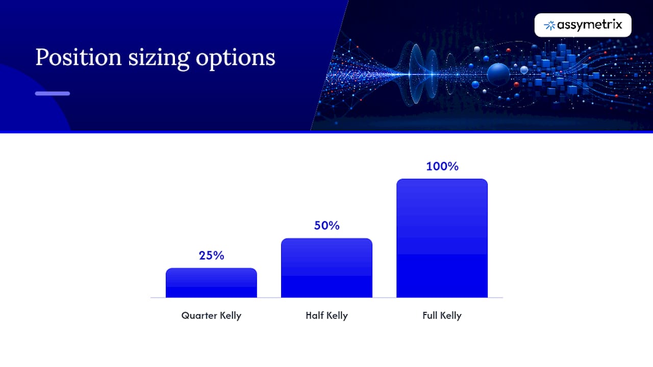
Size positions using fractional Kelly, typically quarter or half Kelly, rather than full Kelly, since decay estimates carry real uncertainty that full Kelly sizing doesn’t tolerate well.
Set a regression-to-mean trigger that automatically cuts allocation to a signal once its rolling half-life estimate drops below a pre-set threshold.
Portfolio and sizing rules matter as much as the signal itself. Practitioner guides on prediction market strategy consistently recommend fractional Kelly sizing, quarter or half Kelly, paired with explicit cash reserves, precisely because a decaying signal’s variance is harder to estimate than its mean return. Staggering resolution scheduling across multiple markets rather than concentrating capital in a handful of same-day resolutions also reduces the risk that a single bad decay estimate wipes out a disproportionate share of a book.
Monitoring closes the loop. A live half-life dashboard that recomputes your decay estimate on a rolling basis, rather than a static number set at deployment, is the difference between catching decay early and discovering it three months later in a drawdown report. Smart Money wallet alerts, flagging when historically skilled wallets start entering the same markets your signal targets, function as an early warning system: skilled capital arriving usually means your remaining edge window is shorter than your backtest assumed.
Pro Tip: Treat a sudden drop in your live half-life estimate the same way you’d treat a risk limit breach, not as a data anomaly to investigate later. By the time you confirm the cause, the edge is usually already gone.
Applied Example: Computing Half-Life With Cross-Venue Data
Running the half-life recipe end to end requires a dataset with specific structural properties, and most public prediction market data falls short on at least one of them. Here’s what a reproducible test actually needs.
Canonical market IDs that map equivalent contracts across Polymarket, Kalshi, and Limitless to a single entity, so cross-venue divergence and arbitrage windows can be measured directly rather than approximated.
Timestamped trade-level data with second-level (or finer) precision, since execution latency effects get washed out at coarser granularity.
Order-book depth snapshots at multiple price levels, not just top-of-book, to compute spread compression accurately.
Wallet-level identifiers on trades, enabling Smart Money cluster detection as an independent decay signal.
Assymetrix maintains 900M+ indexed events dating back to September 2020 across Polymarket, Kalshi, and Limitless, along with over 200 million price snapshots suited to exactly this kind of backtest, according to the company’s own documentation. That depth matters specifically because a half-life estimate built on six months of data carries much wider confidence intervals than one built on multiple years spanning several market cycles and liquidity regimes.
A reproducible test outline looks like this:
Stage | Action | Output |
|---|---|---|
Data pull | Query canonical-ID-aligned trades, order books, and wallet flows across all three venues for the target market category | Unified panel dataset |
Lagged-signal backtest | Simulate signal entry at multiple lags (t+1, t+7, t+14) post-generation | Lagged P&L series |
Half-life fit | Fit exponential decay to lagged P&L, extract decay rate and half-life | Half-life estimate with confidence interval |
Robustness checks | Re-run with purged CV, segment by liquidity tier, apply DSR correction | Adjusted half-life, PBO score |
The Assymetrix backtesting guide walks through the snapshot structure and canonical ID methodology in more detail, and it’s the natural reference point once you’re ready to move from a conceptual outline to actual query design against the API.
What Quants Should Prioritize First
The single biggest mistake in this space is scaling live capital before establishing a reproducible half-life measurement. A statistically fragile edge sized aggressively decays into a loss faster than a modest edge sized conservatively decays into irrelevance, and most quants only discover which situation they’re in after the drawdown.
There’s also a real trade-off between chasing execution speed and chasing model sophistication, and speed usually wins. A marginally better model deployed with high latency loses more edge to decay than a mediocre model deployed fast, because latency cost compounds every single trade while model improvements only help on the margin. Infrastructure investment is not a secondary concern behind signal research. In prediction markets specifically, it’s often the higher-leverage spend.
If you’re picking a first pilot, two options stand out: build a cross-venue arbitrage scanner to get direct experience with how fast structural windows close in practice, or run a Smart Money wallet replication study to see how quickly copying skilled wallets erodes as more capital follows the same trail. Both will teach you more about your own signal’s likely half-life than another quarter of pure backtesting.
— Dean
Put Deep Cross-Venue Data Behind Your Decay Research
Every measurement recipe in this piece depends on one thing: data deep and clean enough to fit a half-life curve you can actually trust. The Assymetrix Data API gives you that foundation, with 900M+ indexed events going back to September 2020 across Polymarket, Kalshi, and Limitless, normalized under canonical IDs so cross-venue comparisons don’t require you to build your own reconciliation layer first.

A reasonable starting experiment: pull two years of tick data for a single market category, run the lagged-signal backtest outlined above, and fit your first half-life curve segmented by liquidity tier. For Polymarket-specific market structure and contract coverage, the Polymarket data resources page is a useful reference point while you scope the pull. From there, the API documentation covers endpoint structure and query patterns for developers building this into an automated pipeline rather than a one-off notebook exercise. Pricing for full API access is available on request through the Assymetrix site.
Sources
The half-life modeling, strategy classification, and validation methods referenced throughout this piece draw on a mix of academic and practitioner sources worth reviewing directly if you’re building your own decay research pipeline.
FAQ
What Is Alpha Half-Life in Prediction Markets?
Alpha half-life is the time it takes for a trading signal’s excess return over a baseline to fall to 50% of its initial value. A modeling paper on AI-driven algorithmic homogenization shows these half-lives compressing from multi-year scales to months as AI adoption among traders increases.
Why Do Some Prediction Market Signals Decay Faster Than Others?
Simple value-betting signals, where an edge comes from disagreeing with the market’s implied probability, tend to decay fastest because they’re easy for other traders to replicate once discovered. Structural strategies like combinatorial arbitrage and passive liquidity underwriting, documented in prediction market strategy guides, decay more slowly because they depend on infrastructure and market-design frictions rather than a single piece of information.
How Do I Measure Alpha Decay Using Historical Data?
Run lagged-signal backtests that simulate entry at multiple time lags after signal generation, then fit an exponential decay curve to the resulting P&L series to extract a half-life estimate. Pair that with spread compression tracking and walk-forward validation to confirm the estimate isn’t an artifact of overfitting.
Why Does Deep Historical Data Matter for Alpha Decay Research?
A half-life estimate built on a few months of data carries wide uncertainty because it hasn’t seen multiple liquidity regimes or market cycles. Assymetrix indexes 900M+ events since September 2020 across Polymarket, Kalshi, and Limitless, giving quants the multi-year depth needed to fit stable, cross-validated decay curves.
Does the Assymetrix Data API Support Cross-Venue Decay Research?
Yes. The Assymetrix Data API normalizes trades, order-book snapshots, and wallet flows across Polymarket, Kalshi, and Limitless under canonical IDs, which is the structural requirement for computing cross-venue arbitrage windows and half-life estimates without building a separate reconciliation layer.
Quants: Measure Alpha Decay in Prediction Markets with 900M+ Events
Alpha decay in prediction markets is measurable, usually fast, and getting faster as AI adoption spreads across Polymarket, Kalshi, and Limitless. A profitable signal’s half-life, the time it takes for its edge to fall by half, often compresses to weeks or months rather than years once capital and copy-trading bots find it. The first move for any quant is not to trade the signal harder. It’s to compute its half-life using lagged-signal backtests built on high-frequency, cross-venue historical data.
TL;DR:
Alpha decay in prediction markets is driven by crowding, rapid information diffusion, and AI homogenization, which can shrink half-lives from years to months.
High-liquidity markets and those with intense attention see the fastest decay, often within hours or days, while niche markets can preserve edges for longer periods.
Accurate measurement of decay requires deep, cross-venue data, precise timestamps, order-book depth, and wallet flow analysis to reliably estimate half-lives.
Running robust backtests with cross-validation and segmenting by liquidity tier is essential to avoid overestimating the persistence of trading edges.
Operational practices such as low-latency data pipelines, diversified timing, and monitoring live half-life dashboards can extend the practical lifespan of profitable signals.
Assymetrixassymetrix.comBuild On Unified Market IntelligenceAccess cross venue prediction market data, Smart Money tracking, and historical trading activity through one integration.Explore Assymetrix
Table of Contents
What Alpha Decay Means in Prediction Markets
Liquidity, Attention, and Market Design Set the Decay Clock
How to Measure Alpha Decay With Historical Prediction Market Data
What the Data Shows About Decay Speed and Strategy Persistence
Mitigation: Operational Practices That Slow the Clock
Applied Example: Computing Half-Life With Cross-Venue Data
What Quants Should Prioritize First
Put Deep Cross-Venue Data Behind Your Decay Research
Sources
What Alpha Decay Means in Prediction Markets
Alpha decay describes the rate at which a signal’s forecasting edge, its ability to beat the market-implied probability, erodes as more capital and faster competitors act on the same information. In prediction markets, this shows up as shrinking realized P&L per contract, tightening bid-ask spreads around the signal’s trigger condition, and probability convergence that happens earlier relative to the resolution date.
The standard way to quantify this is the alpha half-life: the number of trading periods it takes for a signal’s excess return (relative to a naive baseline, like the market’s own implied probability) to fall to 50% of its initial value. If a signal generates 8 cents of edge per dollar risked in week one and only 4 cents by week six, its half-life is roughly six weeks. That number becomes the anchor for every capital allocation and infrastructure decision that follows.
Several causal channels drive decay speed in prediction markets specifically, and they don’t all move at the same pace.
Crowding: as more traders and bots identify the same mispricing, order flow narrows the gap between model probability and market price faster than in equities, where position limits and custody friction slow replication.
Information diffusion speed: prediction markets resolve on discrete, often newsworthy events, so information that used to take days to price in (a polling shift, a court ruling, a company earnings leak) now gets absorbed in minutes on high-attention markets.
Execution latency: the gap between signal generation and order placement matters more in binary markets, where price moves in a fixed 0 to 100 range and small latency costs consume a larger share of a thinner theoretical edge.
AI-driven homogenization: as autonomous agents and LLM-based traders converge on similar features and news-parsing pipelines, they tend to price the same information the same way, at the same time, which compresses the window during which a proprietary signal is actually proprietary. Recent modeling work on AI-driven algorithmic homogenization shows this effect pushing signal half-lives down from multi-year scales to a matter of months in high-adoption regimes.
Fee and market-design effects: maker/taker fee structures, resolution mechanics, and settlement lag all change the breakeven threshold for a signal, meaning a strategy that looked profitable gross can be economically dead net of fees well before its raw statistical edge disappears.
Prediction markets carry structural quirks that don’t exist in most other asset classes. Binary payouts mean a signal’s value is bounded and convex near resolution, so decay isn’t linear. It often accelerates sharply in the final days before settlement as uncertainty collapses. Capital gets locked until resolution, which means a decaying edge still ties up funds that could be redeployed elsewhere, an opportunity cost that rarely shows up in a simple P&L chart. And resolution dates create a hard stop, unlike equities or futures, so a strategy’s effective sample size per market is small, which makes decay estimates noisier and demands more markets, not just more time, to measure reliably.
This is why treating alpha decay as a generic “edge gets arbitraged away” story undersells what’s actually happening. The decay curve in prediction markets is shaped by discrete event structure, binary convexity, and a settlement deadline that traditional decay models built for continuous markets don’t account for. A quant importing a standard equity alpha-decay framework without adjusting for these features will systematically misestimate half-life, usually by overstating it.
Liquidity, Attention, and Market Design Set the Decay Clock
Decay speed is not uniform across venues or market types. It’s a function of how much attention and capital a given market attracts, and how the venue’s fee and settlement structure shapes net returns.
High-liquidity, high-attention markets, major election contracts, marquee sports outcomes, headline macro events, tend to decay fastest. These are exactly the markets where retail flow, market-making bots, and AI agents concentrate, so any mispricing gets closed within hours or days rather than weeks. Low-liquidity niche markets, obscure regulatory outcomes, thinly traded sports props, or long-tail geopolitical questions, can preserve a genuine edge for considerably longer, simply because fewer participants are watching closely enough to correct it.
Liquidity depth acts as a proxy for competition intensity: thin order books with wide spreads usually signal fewer sophisticated participants, which slows decay.
Attention (proxied by volume spikes, social mentions, or news coverage) accelerates decay independent of liquidity, since attention draws in fast-moving arbitrageurs even in moderately liquid markets.
Fee structures compress net edge directly. A signal generating 3% gross edge against a 1.5% round-trip fee burden has a much shorter economically viable life than the same signal on a lower-fee venue, even if the gross statistical edge decays at an identical rate.
Timing around specific events matters as much as venue selection. New market listings create a short window of genuine inefficiency because pricing hasn’t yet absorbed the full available information set, and few bots have built coverage for a market that only just launched. News windows produce a similar but shorter-lived effect: a market can be efficiently priced for days, then suddenly inefficient for a few hours after a surprise headline, before snapping back to efficiency once enough capital reacts. Measuring decay around these windows specifically, rather than averaging over a market’s entire lifespan, gives a much sharper read on where actual exploitable edge sits.
The practical implication is that half-life is not a single number for “prediction markets” as an asset class. It is a distribution that depends heavily on the specific market’s liquidity tier and attention profile. Reporting a blended half-life across venue types without segmenting by liquidity tier will hide exactly the variation a quant needs to allocate capital intelligently.
The Assymetrix liquidity metrics guide covers order-book depth measures that work well as decay-speed proxies, since top-of-book depth and spread width both correlate with how quickly a given market absorbs new information.
How to Measure Alpha Decay With Historical Prediction Market Data
Measuring decay rigorously requires a specific toolkit, not a single backtest. The core metric is the alpha half-life calculation: take a signal’s realized edge in rolling windows after generation, normalize against a lag-zero baseline, and fit an exponential decay curve to the P&L degradation across lagged windows (signal generated at t, position entered at t+1, t+7, t+14, and so on). The decay rate parameter from that fit gives you the half-life directly.
Several auxiliary metrics round out the picture:
Spread compression: track how the bid-ask spread around your signal’s trigger price narrows over the days following signal generation. A market that starts at a 4 cent spread and compresses to 1 cent within a week is telling you competitors found the same edge fast.
Brier score drift: if your signal produces probability forecasts, compute Brier scores across rolling time windows. Rising Brier scores over successive market cohorts indicate your model’s calibration is degrading relative to the market’s own pricing, a direct sign of decaying informational advantage.
Live-versus-backtest equity decay: compare your live P&L curve against the backtested equity curve for the same signal, same period. A growing gap is decay in action, not noise.
Walk-forward performance retention: what percentage of in-sample Sharpe or hit rate survives in out-of-sample walk-forward windows. Retention below roughly 50% across successive folds is a strong decay signal.
PBO and DSR corrections: the Probability of Backtest Overfitting and Deflated Sharpe Ratio adjust for the number of strategy variants tested, correcting for the fact that naive backtests systematically overstate edge persistence when many parameter combinations were tried.
The experimental design that ties these together runs in five stages. First, pre-process the data: align every venue’s market IDs to a canonical schema so a Polymarket contract and its Kalshi or Limitless equivalent on the same underlying event are treated as one entity, not three unrelated series. Second, run lagged-signal simulation: generate the signal at time t using only information available at t, then simulate entries at multiple lags to build the decay curve. Third, apply purged cross-validation, removing training samples that overlap in time with test samples, which prevents leakage that would otherwise make decay look slower than it is. Fourth, run walk-forward validation across sequential out-of-sample periods rather than a single train-test split. Fifth, fit a rolling half-life estimate that updates as new data arrives, so the decay measurement itself adapts rather than staying frozen at a single historical estimate.
The Turbine quant playbook makes a similar case for walk-forward and DSR-adjusted testing as standard practice, not an optional refinement, when validating live persistence claims.
Running this pipeline requires specific data fields: tick-level trade snapshots with timestamps precise enough to sequence events correctly, order-book depth at multiple price levels (not just best bid/ask), maker/taker flags to separate passive from aggressive flow, and wallet-level flow data to identify Smart Money clusters whose entry timing often marks the point where a signal’s remaining life gets short.
Pro Tip: Run your half-life fit separately for each liquidity tier in your universe. A single blended estimate across high-volume and thin markets will average away the exact variation that tells you where capital should actually go.
What the Data Shows About Decay Speed and Strategy Persistence
Modeling work on AI-driven markets gives the clearest quantitative signal available on how fast this is moving. A recent preprint on algorithmic homogenization models an AI-accelerated decay term and finds signal half-lives collapsing from multi-year timescales to a matter of months once AI adoption among market participants crosses a critical threshold. The paper frames this as a Red Queen effect: as adoption spreads, every trader has to keep improving speed and model sophistication just to hold the returns they already had, not to gain new ones.
On the data: the direction of the finding, AI adoption compressing half-lives, is well supported by the modeling logic even though exact month counts vary by parameter assumptions. Treat the qualitative conclusion as robust and the specific numbers as scenario-dependent.
Practitioner evidence lines up with the theory. Guides covering prediction market trading strategies consistently flag simple value-betting signals, buying an outcome because your model disagrees with the market’s implied probability, as the fastest-decaying category. These edges depend on being early to a mispricing, and once even a handful of well-capitalized bots replicate the same model logic, the mispricing closes.
Strategy classes built around market structure rather than opinion tend to hold up longer:
Combinatorial arbitrage, exploiting pricing inconsistencies across related contracts on the same underlying event, persists longer because it requires monitoring multiple markets simultaneously across venues, a data and infrastructure barrier that limits how many participants can execute it well.
Passive liquidity underwriting, earning the spread by providing consistent two-sided quotes, decays more slowly because its profitability depends on structural market-making economics rather than a specific informational edge that can be replicated once discovered.
Structural inefficiencies tied to fee asymmetries or settlement mechanics between venues persist until a venue changes its design, which happens on a much slower timescale than a single trading signal getting crowded out.
Realized numbers back this pattern. Practitioner summaries covering prediction market arbitrage strategies document multi-million-dollar arbitrage extraction historically, while also noting that these windows have been closing faster as venue maturity and bot coverage increase, consistent with the broader decay pattern documented across strategy types.
Mitigation: Operational Practices That Slow the Clock
You cannot stop alpha decay. You can slow it enough to keep a signal economically viable for longer, and the highest-leverage moves are operational before they’re statistical.
Execution and infrastructure improvements come first because they’re often cheaper to fix than the model itself. A canonical cross-venue feed that normalizes Polymarket, Kalshi, and Limitless data into one schema removes the reconciliation lag that eats into your effective reaction time. Timestamp fidelity matters more than most quants assume: if your data pipeline rounds trade times to the nearest minute, your lagged-signal backtests will systematically misjudge how fast a real edge is closing. Automated execution bots that remove human latency from the entry decision buy back time that would otherwise be lost to decay before a single trade is even placed.
Signal engineering is the second lever. Multi-horizon ensembles, combining fast-decaying opinion signals with slower structural ones, smooth out the portfolio-level decay curve even when individual components decay unevenly. Prioritizing structural inefficiencies, arbitrage and market making, over single-event opinion bets shifts your book toward the strategy classes that have historically shown more persistence. Feature regularization matters here too: an overfit model that looks great in-sample often decays faster in practice because its apparent edge was partly noise, not signal, and noise has no half-life worth measuring.
Build or subscribe to a canonical cross-venue feed before optimizing any single-venue signal further.
Rebuild your backtest with purged cross-validation and re-check your half-life estimate; if it drops sharply, your original estimate was contaminated by leakage.
Segment your signal universe by liquidity tier and compute separate half-lives for each.
Size positions using fractional Kelly, typically quarter or half Kelly, rather than full Kelly, since decay estimates carry real uncertainty that full Kelly sizing doesn’t tolerate well.
Set a regression-to-mean trigger that automatically cuts allocation to a signal once its rolling half-life estimate drops below a pre-set threshold.
Portfolio and sizing rules matter as much as the signal itself. Practitioner guides on prediction market strategy consistently recommend fractional Kelly sizing, quarter or half Kelly, paired with explicit cash reserves, precisely because a decaying signal’s variance is harder to estimate than its mean return. Staggering resolution scheduling across multiple markets rather than concentrating capital in a handful of same-day resolutions also reduces the risk that a single bad decay estimate wipes out a disproportionate share of a book.
Monitoring closes the loop. A live half-life dashboard that recomputes your decay estimate on a rolling basis, rather than a static number set at deployment, is the difference between catching decay early and discovering it three months later in a drawdown report. Smart Money wallet alerts, flagging when historically skilled wallets start entering the same markets your signal targets, function as an early warning system: skilled capital arriving usually means your remaining edge window is shorter than your backtest assumed.
Pro Tip: Treat a sudden drop in your live half-life estimate the same way you’d treat a risk limit breach, not as a data anomaly to investigate later. By the time you confirm the cause, the edge is usually already gone.
Applied Example: Computing Half-Life With Cross-Venue Data
Running the half-life recipe end to end requires a dataset with specific structural properties, and most public prediction market data falls short on at least one of them. Here’s what a reproducible test actually needs.
Canonical market IDs that map equivalent contracts across Polymarket, Kalshi, and Limitless to a single entity, so cross-venue divergence and arbitrage windows can be measured directly rather than approximated.
Timestamped trade-level data with second-level (or finer) precision, since execution latency effects get washed out at coarser granularity.
Order-book depth snapshots at multiple price levels, not just top-of-book, to compute spread compression accurately.
Wallet-level identifiers on trades, enabling Smart Money cluster detection as an independent decay signal.
Assymetrix maintains 900M+ indexed events dating back to September 2020 across Polymarket, Kalshi, and Limitless, along with over 200 million price snapshots suited to exactly this kind of backtest, according to the company’s own documentation. That depth matters specifically because a half-life estimate built on six months of data carries much wider confidence intervals than one built on multiple years spanning several market cycles and liquidity regimes.
A reproducible test outline looks like this:
Stage | Action | Output |
|---|---|---|
Data pull | Query canonical-ID-aligned trades, order books, and wallet flows across all three venues for the target market category | Unified panel dataset |
Lagged-signal backtest | Simulate signal entry at multiple lags (t+1, t+7, t+14) post-generation | Lagged P&L series |
Half-life fit | Fit exponential decay to lagged P&L, extract decay rate and half-life | Half-life estimate with confidence interval |
Robustness checks | Re-run with purged CV, segment by liquidity tier, apply DSR correction | Adjusted half-life, PBO score |
The Assymetrix backtesting guide walks through the snapshot structure and canonical ID methodology in more detail, and it’s the natural reference point once you’re ready to move from a conceptual outline to actual query design against the API.
What Quants Should Prioritize First
The single biggest mistake in this space is scaling live capital before establishing a reproducible half-life measurement. A statistically fragile edge sized aggressively decays into a loss faster than a modest edge sized conservatively decays into irrelevance, and most quants only discover which situation they’re in after the drawdown.
There’s also a real trade-off between chasing execution speed and chasing model sophistication, and speed usually wins. A marginally better model deployed with high latency loses more edge to decay than a mediocre model deployed fast, because latency cost compounds every single trade while model improvements only help on the margin. Infrastructure investment is not a secondary concern behind signal research. In prediction markets specifically, it’s often the higher-leverage spend.
If you’re picking a first pilot, two options stand out: build a cross-venue arbitrage scanner to get direct experience with how fast structural windows close in practice, or run a Smart Money wallet replication study to see how quickly copying skilled wallets erodes as more capital follows the same trail. Both will teach you more about your own signal’s likely half-life than another quarter of pure backtesting.
— Dean
Put Deep Cross-Venue Data Behind Your Decay Research
Every measurement recipe in this piece depends on one thing: data deep and clean enough to fit a half-life curve you can actually trust. The Assymetrix Data API gives you that foundation, with 900M+ indexed events going back to September 2020 across Polymarket, Kalshi, and Limitless, normalized under canonical IDs so cross-venue comparisons don’t require you to build your own reconciliation layer first.
A reasonable starting experiment: pull two years of tick data for a single market category, run the lagged-signal backtest outlined above, and fit your first half-life curve segmented by liquidity tier. For Polymarket-specific market structure and contract coverage, the Polymarket data resources page is a useful reference point while you scope the pull. From there, the API documentation covers endpoint structure and query patterns for developers building this into an automated pipeline rather than a one-off notebook exercise. Pricing for full API access is available on request through the Assymetrix site.
Sources
The half-life modeling, strategy classification, and validation methods referenced throughout this piece draw on a mix of academic and practitioner sources worth reviewing directly if you’re building your own decay research pipeline.
FAQ
What Is Alpha Half-Life in Prediction Markets?
Alpha half-life is the time it takes for a trading signal’s excess return over a baseline to fall to 50% of its initial value. A modeling paper on AI-driven algorithmic homogenization shows these half-lives compressing from multi-year scales to months as AI adoption among traders increases.
Why Do Some Prediction Market Signals Decay Faster Than Others?
Simple value-betting signals, where an edge comes from disagreeing with the market’s implied probability, tend to decay fastest because they’re easy for other traders to replicate once discovered. Structural strategies like combinatorial arbitrage and passive liquidity underwriting, documented in prediction market strategy guides, decay more slowly because they depend on infrastructure and market-design frictions rather than a single piece of information.
How Do I Measure Alpha Decay Using Historical Data?
Run lagged-signal backtests that simulate entry at multiple time lags after signal generation, then fit an exponential decay curve to the resulting P&L series to extract a half-life estimate. Pair that with spread compression tracking and walk-forward validation to confirm the estimate isn’t an artifact of overfitting.
Why Does Deep Historical Data Matter for Alpha Decay Research?
A half-life estimate built on a few months of data carries wide uncertainty because it hasn’t seen multiple liquidity regimes or market cycles. Assymetrix indexes 900M+ events since September 2020 across Polymarket, Kalshi, and Limitless, giving quants the multi-year depth needed to fit stable, cross-validated decay curves.
Does the Assymetrix Data API Support Cross-Venue Decay Research?
Yes. The Assymetrix Data API normalizes trades, order-book snapshots, and wallet flows across Polymarket, Kalshi, and Limitless under canonical IDs, which is the structural requirement for computing cross-venue arbitrage windows and half-life estimates without building a separate reconciliation layer.
Other Blog


